The falling motion of a boulder along a rocky slope depends on many factors that are not easy to express numerically.
The trajectories of the boulders depend on the geometry of the slope, on the shape of the falling boulder and on its initial velocity at the moment of detachment from the slope, and also on the entity of the energy dissipated due to the impacts during the fall. The falling boulders can slide, roll or bounce downstream depending on their shape, flattened or rounded, and on the gradient of the slope.
The energy dissipated due to impacts is generally different and varies with the characteristics of the motion and depends on the mechanical characteristics of the boulder and on the materials present along the slope (rock, soil, vegetation) that oppose in a different manner to the motion of the boulders.
In reality, however, it is practically impossible to determine precisely the contour of a slope and detect the shape of the different boulders that may detach.
In addition, the geometry of the slope and the nature of the outcropping materials undergo changes over time, sometimes sensitive, as a result of the alteration of the rock, of the accumulation of debris in the less steep areas and of the development of the vegetation.
Finally, it is practically impossible to model the motion of boulders fall in cases in which these shatter due to impacts, nor is it possible to identify the areas of the slopes where shatter occurs.
For the analysis of the falling trajectories we need to refer to very simplified models: the geotechnical design of the protection interventions must be, therefore, developed on the basis of a large numerical experimentation, making it possible to explore the different aspects of the phenomenon and recognize the main factors that affect the motion of fall in the particular situation in question.
In more complex cases it might be necessary to calibrate the model on the basis of an analysis of trajectories detected by in situ cinematography following the collapse of the boulders.
There are two analytical models, Lumped-Mass and Colorado Rockfall Simulation Program (CRSP), used mainly to study the phenomenon of rock fall in an analytical way. In the Lumped-Mass model the falling boulder is considered as a simple point having a mass and velocity, and the impact on the ground is affected by the normal and tangential restitution coefficients. A more rigorous model is, however, the CRSP, as it takes into account the shape and size of the boulder.
Lumped Mass Method
By choosing this option, the computation of the trajectories is made with the Lumped Mass method (hypothesis of point boulder).
CRSP Method
By choosing this option, the computation of the trajectories is made with the Colorado Rockfall Simulation Program method (hypothesis of three-dimensional boulder).
Calculate
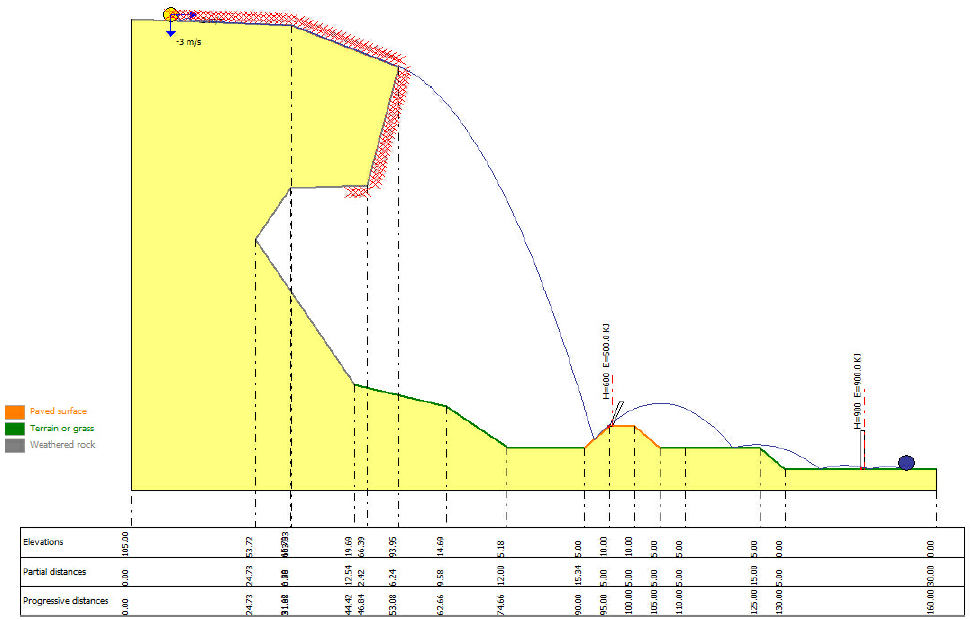
The calculation is based on the method chosen by viewing the trajectories followed by the boulder on the basis of its dimensions and of the restitution coefficients. When the calculation is performed in the side panel of the work area is shown the information on individual trajectories: order number, representation color, description and maximum abscissa reached.
Option for the visualization of trajectories defined in the calculation. To display, proceed as follows:
•Choose "Show single trajectories".
•On the side panel, choose the trajectory to be displayed on the screen.
•Select a single trajectory clicking in the grid on the trajectory to display.
•Move the mouse over the work area: scrolling the mouse cursor along the trajectory on the status bar (the bar at the bottom of the worksheet) will be shown the values of the velocity of the boulder, the height of the trajectory and the energy of the boulder.
•For the chosen trajectory, in the grid below, a discretization of the trajectory is carried out at a constant pitch and, for each abscissa X, is returned to the flight time, the height of the trajectory at point X, the velocity and energy of the boulder. The data grid can be copied and pasted into Excel.
•Moreover, in correspondence of the single trajectory, with the data reported in the table, the program allows the generation of graphics of heights, velocity and energy. These charts are created directly on the section and can be printed with the command "Print Preview".
Info on single trajectories
By selecting this option, the user can get information on individual trajectories. To do so, proceed as follows:
•On the grid "Show single trajectories", select the path to be displayed.
•Scroll with the mouse over the points of the selected trajectory, it will open a label that will show step by step the values of impact velocity, the height of the parabola with respect to the profile of the slope, the fraction of flight time in that point and the value of the kinetic energy of the boulder in that point.
Report for % boulders not passing
Returns the values of % of boulders intercepted at each abscissa. Selecting this command is displayed a dialog box in which it is required the scanning step of the horizontal axis: each X shows the percentage of stopped boulders, and, by selecting the option "Show Mesh % stopped boulders" are shown the corresponding percentages along the path of the boulder.
Graphic parameters
In this panel can be configured the settings for the proper display of the graphics given below. In particular, for the "Energy histogram" can be chosen the representation step of the energy by typing the value in the "Display step" field, or set the program to define it automatically. For "Energy distribution" can be chosen the step with which to vary the abscissa where is computed the energy of the boulder and the representation factor of the energy for a more or less scaled view of the peaks. For the "Parabola graphic", similarly, must be set the representation factor for a more or less pronounced view of the height peaks.
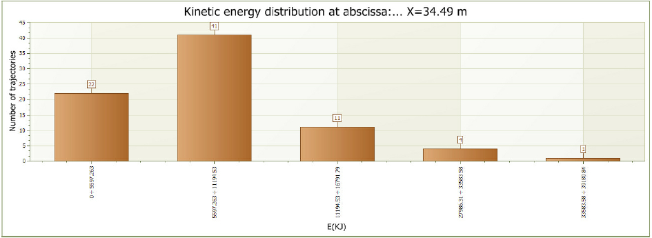
The command builds a histogram which shows the distribution of the trajectories' energy at a particular point defined by the user.
On the abscissa are represented energies at intervals, while on the ordinate the number of trajectories that have an energy value of in one of the intervals in which it was discretized the abscissa axis.
To choose the point at which to calculate the energy the user must move on the work area and with a on a specific point. A table will appear asking the user to confirm or change the abscissa of the chosen point. After the confirmation the energy histogram is regenerated with the values of the corresponding energies.
The generation of the histogram is available after performing the computation.
The histogram can be copied to the clipboard and pasted as a bitmap: go on the histogram and press the right mouse button. From the menu the user can also choose to do a print preview and optionally print the graphic.
Represents, for each trajectory, the trend of the boulder's energy along the fall path. On the abscissa is represented the X (progressive distance along the profile), while on the ordinate is represented the energy of the boulder in the considered point. After performing the computation, a right click brings up a selection window from which the user can choose the graphic to be displayed on the screen. The user is given the opportunity to make a choice on viewing single trajectory or view all the energy graphics associated to each trajectory. The representation of the set of graphics is done in sequence from left to right; for full view just move anywhere on the graphic and with the left mouse button scroll from right to left.
On the axes of the Cartesian reference system is present the scrollbar to move from left to right and from bottom to top on the Cartesian plane. This functionality is activated when the scale of graphical representation does not allow to obtain a complete representation of the graphic on the work area. The "Envelope" command is used to represent the set of all graphics of the energy associated with individual trajectories.
The user has the possibility to choose whether to display the labels with the values on the graphic. The option is activated with a right click , "Labels."
The graphics can be copied into memory to be subsequently pasted into Word or other applications, the user can also view the print preview of the work area. All operations can be performed by selecting the specific command after a right click.
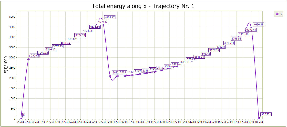
with labels
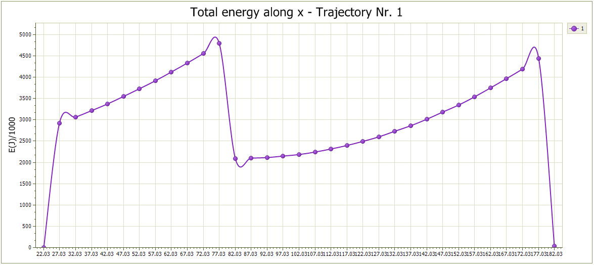
without labels
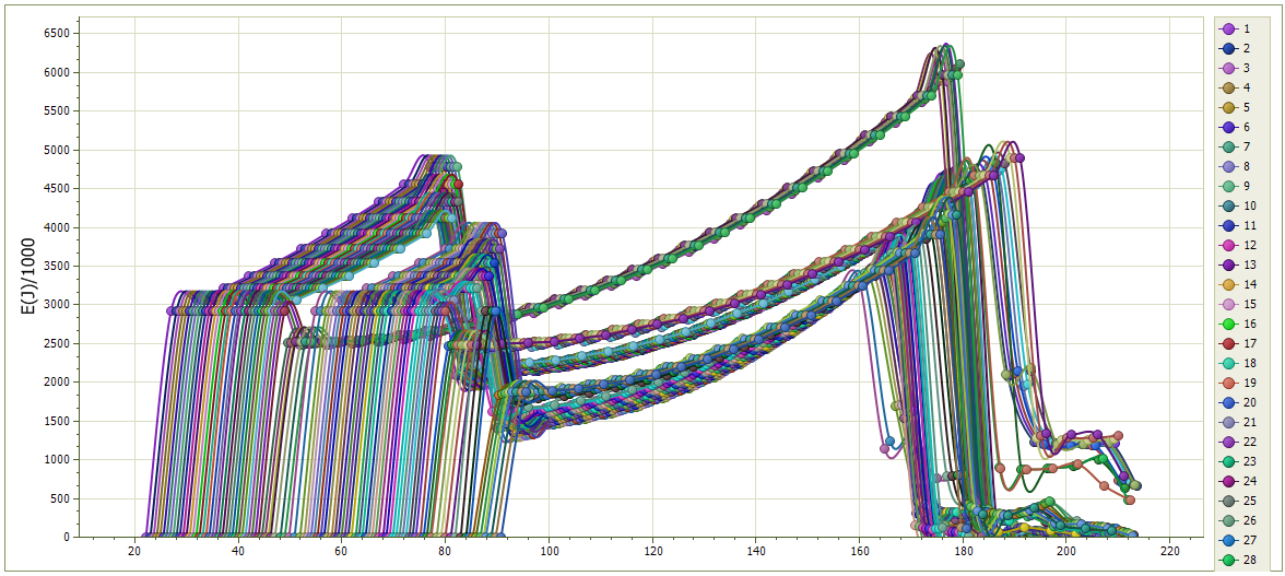
envelope
Trajectories graphic or parabolas' heights graphic, is the trend of the boulder's height along the fall path. On the abscissa is represented the X (progressive distance along the profile), while on the ordinate is represented the height of the boulder in the specific point. The graphic can be displayed using the same basis set out in the section "Energy distribution graphic".
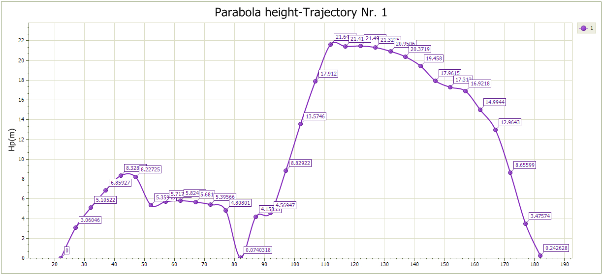
with labels
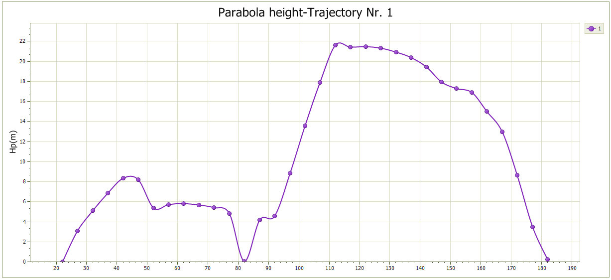
without labels
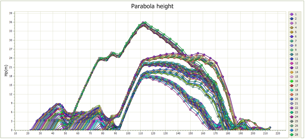
envelope
Backfill
The template allows the user to create protection barriers (backfill). To insert them on the profile just confirm the assigned dimensions with "Ok", go on the work area with and choose the specific point of insertion with a simple click.
© GeoStru