Premise

The program GMS (GeoMechanical Survey) has the aim to represent and process the geo-structural survey of rock masses joints performed in-situ with the method of the compass and clinometer, according to the ISRM recommendations.

The joints in a rock mass condition, in a more or less evident way, the mechanical behavior of the rock and of the geotechnical model at the basis of any calculation. It is important, in order to correctly evaluate the stability condition, to have a precise description of the rock structure and joints, both in qualitative and quantitative terms.

For the determination of the rock's geotechnical model will be, therefore, illustrated the stages of joints survey, referring to geo-structural conditions (spacing, aperture, persistence) and to hydraulic and joint strength conditions (roughness, wall strength, degree of alteration, filling materials).

The procedure used for performing the survey is described in the ISRM recommendations, "Suggested Methods for the Quantitative Description of Discontinuities in Rock Masses."

Survey of discontinuity

Discontinuity

Is the general term for any break in the continuity of a rock mass having low or no tensile strength. Is the collective term for the majority of the cracks, of the stratification planes, of the schistosity planes, of the weakening zones and of faults.

The ten parameters chosen in the ISRM Recommendations to describe the discontinuities and the rock masses are defined as follows:

Orientation

Position of the discontinuity in space. The surfaces of discontinuity may be represented as a plane whose joint is identified by a pair of angles (α, β) or (α, γ), where α is the inclination, γ the direction and β the azimuth of the discontinuity (in Anglo-Saxon terminology , respectively, dip , strike and dip direction referred to a plan).

The instrumentation used is equipped with a compass having an air bubble level and a flat lid, which is resting on the surface of discontinuity causing it to rotate around a horizontal axis (clinometer).

The maximum inclination of the discontinuity's middle plane α (dip) is measured with the clinometer and is expressed in degrees with two-digit numbers from 00 ° to 90 °.

The azimuth of the immersion β (dip direction) is measured in degrees counted clockwise from the North and is expressed as a three-digit number from 000 ° to 360 °.

The couple (dip, dip direction) represents the immersion vector.

The field measurements are performed along a sampling line, materialized on the rocky front with metric strip fixed at the ends of the relief, and so are detected all the discontinuities encountered proceeding from one end to another.

Spacing (S)

Distance between adjacent discontinuities measured in the direction orthogonal to the discontinuities them self. Normally it refers to the average or modal spacing of a cracks system. Together with the orientation and the persistence determines the shape and size of the blocks in which is divided the rock mass. Since the measure d, expressed in cm, is performed orthogonally to the discontinuity, must be adjusted taking into account of the angle δ between the joint and the sample line: S = d sin δ.

For each family is defined a frequency distribution that can be represented on histograms. The distribution of the spacing is at the base of the ISRM classification shown in Table 1.

Description	Spacing
Extremely narrow spacing	< 2 cm
Very close spacing	2÷6 cm
Narrow spacing	6÷20 cm
Moderate spacing	20÷60 cm
Wide spacing	60÷200 cm
Very wide spacing	200÷600 cm
Extremely large spacing	> 600 cm

Tab.1: ISRM classification according to the spacing

Continuity or persistence

Length of the discontinuity observed in outcrop. Can give a rough measure of the areal extent or penetration depth of a discontinuity. The fact that the plane of discontinuity ends in massive rock or against other discontinuities, reduces the persistence. In Table 2 is shown the ISRM classification as a function of persistence.

Description	Persistence
Very low persistence	<1 m
Low persistence	1÷3 m
Average persistence	3÷10 m
High persistence	10÷20 m
Very high persistence	>20 m

Tab.2: ISRM classification according to the persistence

Roughness

Roughness of facing surfaces of a discontinuity and undulation relatively to the median plane of the discontinuities. Both the roughness and its morphological evolution contribute to shear resistance, especially in the case of interconnected structures and without relative displacements.

The importance of the roughness decreases with the increase of the aperture of the same discontinuity.

In general terms, the roughness can be characterized by an undulation and by a genuine and real roughness. In the first case the shape of the undulation causes the dilatancy in case of cross sliding. In the second case the form of the roughness tends to be broken in case of sliding .

The methodology and instrumentation to perform the survey are shown in the ISRM Recommendations that are mentioned below.

The roughness can be detected in two different ways :

1.If is known the direction of potential sliding, the roughness can be detected with linear profiles chosen parallel to this direction. In many cases, the sliding direction is parallel to the dip direction. In cases in which the sliding is conditioned by two intersected, different planes of discontinuity, the direction of potential sliding is parallel to the planes intersection line. In the case of stability for a shoulder of an arch dam, the direction of the potential sliding can have a significant horizontal component.

2.In case is not known the direction of potential sliding, but it is very important to know it, the roughness can be measured in three dimensions instead of two. This can be done with a compass and a disc clinometer. The readings of the inclination and direction can be rendered graphically as poles on equal area lattices. Alternatively, the discontinuity surfaces can be detected using the photogrammetric method. This can be a useful technique when the critical surfaces are inaccessible.

The aim of all methods of roughness measuring is the assessment or calculation of the shear strength and dilatancy. The interpretation methods of the roughness profiles and the estimation of the shear strength currently available are illustrated in the following point.

Instrumentation

The detection method of the linear profile of roughness requires the following equipment:

1. folding rod of at least two meters, marked in mm

2.compass and clinometer

3.ten meters of fine wire or nylon wire, marked at intervals of one meter (in red) and one decimeter (in blue)

The ends of the wire should be attached to blocks of wood or similar, so that it can be stretched to form a reference line straight above the large undulation discontinuity plan.

The roughness detection method using compass and clinometer disc requires the following equipment:

1.a geological compass Clar (Breithaupt) with a horizontal built-in bubble level and a rotating lid joined to the main body of the compass by a marked hinge to measure the inclination

2.four thin circular disks in light alloy, of various diameters (ex. 5, 10, 20, 40 cm), which may be fixed from time to time to the lid of the compass [see ISRM bibliography].

Procedure

Linear profile

The discontinuities are chosen in such a way as to be accessible and typical for the surface of potential scrolling.

Depending on the size of each plane, will be used the marked rod of 2 meters or the wire of l0 meters, placing them above the discontinuity plane, parallel to the direction of the potential sliding. They should be placed at the contact point or points with the highest elevation and should also be as straight as possible. A thin layer of plasticine can be used to prevent the sliding of the rod downwards along the line of maximum inclination. The dough can be placed between the rod and the ridges of the discontinuity. Are measured the distances (y) on the perpendicular between the rod (or wire) and the surface of the discontinuity, to the nearest mm, for given tangential distances (x).

It is advisable to be flexible in the choice of "x", since a regular interval (ex. 5 cm) could make neglecting a small step or something like that might be of importance in the evaluation of shear strength. In general, values of (x) equal to approximately 2% of the total measured length, are enough to obtain a substantially good measure of the roughness.

The (x) and (y) are tabulated together with the azimuth and inclination of the measurement base. They may be different from the orientation dip/dip direction of the discontinuity.

The typical profiles of the minimum, average and maximum roughness are detected using the above procedure. They may be referred to a whole discontinuity system, to a critical discontinuity or each measured surface, depending on the required level of detail.

The angle of corrugation (i), shown in Figure 1, should be measured with the rigid rod and the clinometer, if the detected profile is so short that it can not include the entire undulation.

The length and the approximate amplitude of an undulation too large to be measured with the linear profile should be estimated or measured when there are no problems of accessibility .

Photographs depicting surfaces with minimum, average and maximum roughness should be taken with a ruler of 1 meter placed prominently in contact with the surface under examination.

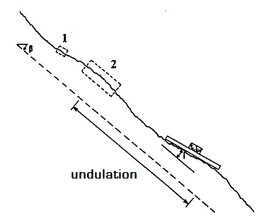
Figure 1

Compass and clinometer disc

The chosen discontinuities must be such as to be accessible and typical for the potential sliding surface. The roughness angles (i) on a small scale (Figure 2) are measured by placing the disc of larger diameter (ex. 40 cm diameter) on the discontinuity surface in at least 25 different positions, and registering both the inclination that the direction of maximum slope for each position. (Is taken into consideration a surface area at least ten times greater than that of the disc of larger diameter).

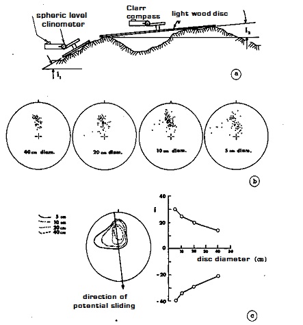
Figure 2

When is not possible to perform the procedures described above, the ISRM Recommendations advise the use of descriptive terms of the roughness that can be summarized in Figure 3.

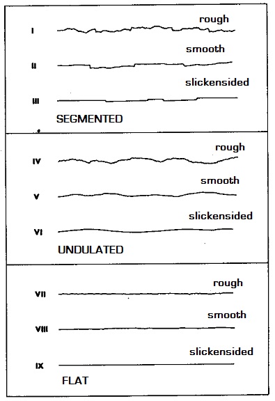
Figure 3

Evaluation of the shear strength

The roughness gives indications for the evaluation of the shear strength of not filled discontinuities.

The peak values of ϕ can be estimated with the relationship:

where:

JRC = joint roughness coefficient

JCS = joint compressive strength of the walls

ϕγ = residual angle of friction

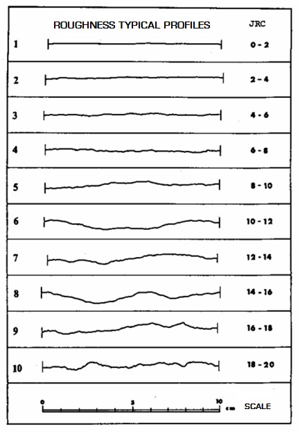
Figure 4

The value of JRC is derived from the graphics in Figure 4, the values of JCS and ϕγ are obtained from the tests with the Schmidt hammer, performed both on the wall of the discontinuity and on a fresh fracture of intact rock material.

Another useful parameter for the classification of the rock is the Jr ("Joint Roughness Number") which depends on the roughness of the joint walls whose values are summarized in Table 3.

Wall strength

Compressive strength equivalent of the facing edges of a discontinuity. It may be less than the strength of the rock mass due to exposure to atmospheric agents or to the alteration of the walls. Constitutes a major component of the shear strength if the walls are in contact.

The effects of atmospheric actions are of two main types: mechanical disintegration and chemical decomposition.

The first occurs with the expansion of pre-existing discontinuity or with the formation of new ones, the opening of inter-granular fractures and breakage of individual minerals.

The second one is manifested by a discoloration of the rock and leads to a decomposition of silicate minerals in clay minerals. In the case of carbonate and saline rocks it is very important the dissolution phenomenon.

	Class	Roughness	Jr
Rock wall contact and rock wall contact before 10 cm shear	A	Discontinuous fractures	4
	B	Rough, irregular, undulating	3
	C	Undulating, smooth	2
	D	Undulating , slickensided	1,5
	E	Planar, rough or irregular	1,5
	F	Planar, smooth	1
	G	Planar, slickensided	0,5
No rock contact when sheared	H	Clay minerals thick enough to prevent rock wall contact	1
No rock contact when sheared	I	Sandy, gravelly or crushed zone, thick enough to prevent rock wall contact	1

Tab.3: Jr coefficient

The wall strength, as seen, can be calculated with the Schmidt hammer and by scratching tests.

Another useful parameter for the classification of the rock is the Ja ("Joint Alteration Number") which depends on the alteration degree of the fractures, the thickness and the nature of the filling. The values are summarized in Table 4:

Class	Alteration of surfaces	Ja
A	Impermeable, hard, tightly healed, non-softening filling	0,75
B	Unaltered joint walls, surface staining only	1
C	Slightly altered joint walls, non-softening mineral coatings, sandy particles, clay-free disintegrated rock	2
D	Silty or sandy clay coatings, small clay fraction	3
E	Softening or low-friction clay mineral coatings	4
F	Sandy particle, clay-free disintegrated rock	4
G	Strongly over-consolidated, non-softening clay mineral fillings	6
H	Medium or low over-consolidation, softening clay mineral filling (continuous, < 5 mm thick)	8
I	Swelling clay fillings	8÷12

Tab.4: Ja coefficient

In the ISRM Recommendation is added another coefficient, W, that varies from 1 (bedrock or little altered) to 6 (extremely altered rock). In the table below is shown the complete classification:

Name	Description	W
Bedrock	There are no visible signs of alteration of the rock material, at most, a slight discoloration on the surface of the major discontinuities	1
Slightly altered	The discoloration indicates an alteration of the rock material and discontinuity surfaces. All the rock material can be bleached and can sometimes be externally less resistant than bedrock within	2
Moderately altered	Less than half of the rock material is decomposed and/or disintegrated as a ground. Bedrock or discolored rock is present either as a continuously spine or within individual blocks	3
Strongly altered	More than half of the rock material is decomposed and/or disintegrated as a ground. Bedrock or discolored rock is present either as a discontinuous spine or within individual blocks	4
Completely altered	All the rock material is decomposed and/or disintegrated as a ground. The massive original structure is still largely intact	5
Residual soil	All the rocky material has become a terrain. The structures of the mass and rock materials are destroyed. There is a strong change in volume but the soil has not undergone significant transport	6

Tab.5: W coefficient

Aperture

Distance between the facing edges of a discontinuity in which the intervening space is filled with air or water.

The thin apertures can be measured with a gauge, while the large ones with a ruler graduated in mm. They are detected along the intersection with the alignment of the survey.

Based on the measurements, the ISRM Recommendations propose the following classification:

Aperture	Description	Discontinuity
<0,1 mm	Very narrow	Closed
0,1÷0,25 mm	Narrow
0,25÷2,5 mm	Partly opened
0,5÷2,5 mm	Opened	Semi-open
2,5÷10 mm	Moderately large
>10 mm	Large
1÷10 cm	Very large	Open
10÷100 cm	Extremely large
> 1 m	Cavernous

Tab.6: ISRM classification according to aperture

Filling

Material that separates the adjacent walls of a joint and that is usually less resistant than primitive rock. Typical filling materials are sand, silt, clay, more or less fine break, mylonite. It also includes thin layers of minerals and welded joint, for example, the veins of quartz and calcite.

The presence of filling material influences the behavior of the joint in respect of the mutual movement of the joint walls. In the survey is indicated the characteristic in reference to its hardness (R: rigid - P: plastic).

Seepage

Flow of water and abundant moisture, visible in the individual discontinuities or in the rock mass as a whole.

The ISRM Recommendations provide descriptive diagrams to estimate the seepage through discontinuity without filling (Table 7), discontinuity with filling (Table 8) and a rock mass (Table 9).

Seepage degree	Description
1	The discontinuity is very closed and dry; water flow along it does not appear possible.
2	The discontinuity is dry without any obvious water flow.
3	The discontinuity is dry but showing obvious signs of water flow, such as traces of oxidation, etc.
4	The discontinuity is moist but there is no free water.
5	The discontinuity shows seepage, occasional water drops but no continuous flow.
6	La discontinuità mostra un flusso continuo di acqua, (stimare la portata in lImino e descrivere se la pressione è bassa, media, o alta). The discontinuity shows a continuous water flow, (to estimate the scale and describe if the pressure is low, medium, or high).

Tab.7: Discontinuity without filling

Seepage degree	Description
1	The filling materials are definitely consolidated and dry; a significant flow appears unlikely because of the very low permeability.
2	The filling materials are moist but there is no presence of free water
3	The filling materials are wet; occasional drops of water
4	The filling materials show signs of leaching; continuous water flow (assess flow rate in l/min).
5	The filling materials are locally leached; considerable water flow along the run-off channels (assess flow rate in l/min and describe the pressure, whether low, medium or high).
6	The filling materials are completely washed out; observed water high pressures especially at exposure time (asses the pressure in l/min and describe pressure)

Tab.8: Discontinuity with filling

Seepage degree	Description
1	Dry walls and crown, no detectable seepage
2	Little seepage, specify dripping discontinuities
3	Average flow; specify the discontinuity with continuous flow (asses flow rate in l/min over a l0 m excavation)
4	High flow, specify the discontinuity with intense flow (asses the flow rate in l/min/l0 m long excavation)
5	Exceptionally high flow; specify the source of this flow, (asses the flow rate in l/min/l0 m long excavation).

Tab.9: Rock mass (ex. contour gallery)

Number of joint sets

Defines the set of existing systems. The rock mass can be further divided by discontinuities of a particular character.

In the survey phase are taken into account all present systems; plotting the poles of the discontinuities and outlining with lines of equal density, the main systems can be obtained.

According ISRM Recommendations, the discontinuities that appear locally can be classified according to Table 10:

Degree	Description
1	massive; occasional and random joints
2	one joint set
3	one joint set plus random
4	two joint sets
5	two joint sets plus random
6	three joint sets
7	three joint sets plus random
8	four or more joint sets
9	crushed rock, earth like

Tab.10: ISRM classification according joint sets

Another useful parameter for the classification of rock mass is Jn ("Joint Set Number") that depends on the number of joint systems present in the rock. The values are summarized in Table 11:

Class	Description	Jn
A	massive, none to few joints	0÷1
B	one joint set	2
C	one joint set plus random	3
D	two join sets	4
E	two join sets plus random	9
F	three join sets	6
G	three join sets plus random	12
H	four or more joint sets, random, heavily jointed, "sugar cube", etc	15
I	crushed rock, earth like	20

Tab.11: Classification according to Jn coefficient

Block size

Block size resulting from the mutual orientation of the fracture systems that intersect and the spacing of the individual systems. Singular joints can further influence the unit rocky volume and its shape.

The index of the blocks size (Ib) represents the average size of the typical rock blocks. Two joint sets perpendicular to each other give a cubic or prismatic form to the blocks. In this case the value of Ib is:

Where S1, S2 and S3 represent the averages of the modal values of individual spacings.

Graphical representation of the joint survey

The graphical representation of the joint can be made in several ways:

1.Wulff diagram

2.Schmidt-Lambert diagram

3.Polar stereographic diagram

4.Polar equal area diagram

5.Star diagram

6.Representation by histograms of the main characteristics (spacing, aperture, persistence)

Wulff diagram

Is the stereographic projection of the terrestrial meridians and parallels on a plane passing through the center and to the two poles. It is a isogonal projection, in which the angles between the individual planes are retained on the projections, for which the areas defined by the intersection between two parallels and two meridians are strongly distorted from the center towards the edges of the lattice.

Schmidt-Lambert diagram

It is used to prevent the areal distortion of the Wulff diagram and therefore suitable for statistical interpretations. The great circles are represented by arcs of ellipses.

Equal area, equiangular and stereographic polar diagram

They are similar to the previous ones, where are represented the joint poles.

Star diagram

Representation of joints' measurements. the observations are represented on a circular reference marked from 0 ° to 360 ° and radial lines at intervals of 10 °. The observations are grouped in 10° sector to which they belong. The number of observations is represented in a radial direction relative to the circles corresponding to 5, 10 and 15 observations.

Isodensity diagram

From the distribution on the poles grid corresponding to a significant data set can be recognized a number of joint families. To achieve this goal are plotted the isodensity diagrams, place of centers of unit areas that contain the same number of poles. The unit area is conventionally equal to 1% of the total area of the diagram.

The method used to investigate the distribution of the poles' density is developed by Denness who has divided the reference sphere in 100 elementary cells .

Projected on the Schmidt diagram, a generic cell assumes a curvilinear contour preserving the area, which contains a certain number of poles. For the construction of the grid, Denness divides the circle according to a number of rings (7 for the type A grid and 6 for type B grid), each ring will contain a number of cells, the number increasing from the center towards the outside of the diagram.

The type A grid is suitable for analysis in which the poles are concentrated in the vicinity of the outer circumference ( subvertical families), while the type B diagram is suited for inclined or subhorizontal surfaces.

Markland test

The purpose of the Markland test is to quantify the possibility of rock wedge failure in which the sliding occurs along the intersection line of two planar joints .

The safety factor of the slope depends on the inclination of the intersection line, on the shear strength of the joint's area and on the geometry of the wedge. The limit case occurs when the wedge degenerates into a plane, that is, the two planes have coincident inclination and immersion and when the shear strength of this plan is only due to friction. The sliding, in these conditions, occurs when the inclination of the plane is greater than the angle of friction and can be performed a preliminary stability check by comparing the inclination of the intersection line of the two planes and the friction angle of the rocky surface. The slope is potentially unstable when the point, in an equal area diagram, which defines the intersection line of the two planes, falls within the area bounded by the great circle that represents the slope and the circle that represents the friction angle.

The test has been implemented to evaluate the critical joints. This test must be followed by more detailed stability analysis.

A further development of the Markland test has been implemented by Hocking. The test in fact provides for the possibility that the sliding occurs along one of the planes that constitute the wedge and not only along the intersection line of the two planes themselves.

In fact, if the Markland test is verified and the immersion of one of the planes falls between the slope's immersion and the direction of the intersection line, the sliding will occur on the plane rather than along the intersection line.

Theoretical notes