The bearing capacity of a shallow foundation can be defined as the maximum value of the load applied, for which no point of the subsoil reaches failure point (Frolich method) or else for which failure extends to a considerable volume of soil (Prandtl method and successive).
Experimental observations have shown that the soil can get to failure through three mechanisms (see image below): General failure is characterized by the formation of well-defined sliding surfaces that start from the foundation and reach the ground level, and a swelling of the soil at the sides of the foundation. Punching failure when the lowering of the foundation is made possible by the formation of vertical shear planes along the perimeter, without generating sliding surfaces. Local failure corresponds to the formation of a clear sliding surface below the foundation, which is dispersed in the adjacent soil, it shows a tendency to swelling timid side of the ground.
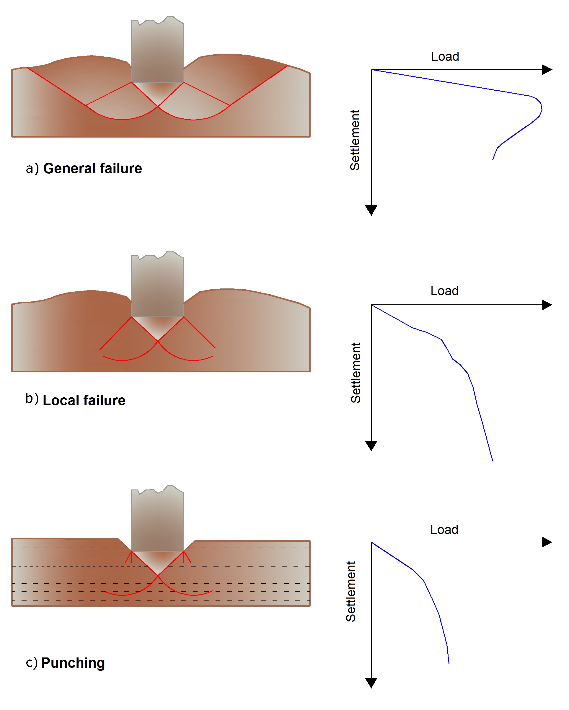
Types of soil failure
The solutions available for the calculation of the bearing capacity are based on the assumption of rigid-plastic behavior of the soil and are therefore, strictly speaking, only applicable to the case of general failure.
It can be shown that the bearing capacity of a soil is the sum of three factors: soil weight γ', q' overload and cohesion c'; solutions available today have been obtained by the superposition of individual independent problems.
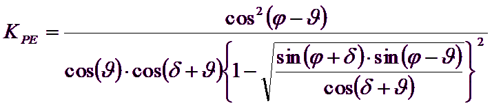
Prandtl (1921) has studied the problem of failure of an elastic half-space due to a load applied on its surface with reference to steel, characterizing the resistance to failure with a law of the type:
|
(1-1) |
valid even for soils.
Prandtl assumes:
•Rigid- plastic behaviour
•Failure resistance of the material expressed with the relationship (1-1)
•Uniform vertical load applied to an infinitely long strip of width 2b (Plane strain case)
•No tangential shear on the interface between load strip and boundary surface of the half-space
•No overload the edges of the foundation (q'=0)
In the space between the upper (where the load lies) and lower (indicated by GFBCD) surface, simultaneously with failure, the plasticization phenomena occurs.
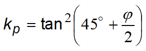
Within the triangle AEB failure occurs according to two families of straight segments inclined by 45°+φ/2 to the horizontal.
Within zones ABF and EBC failure occurs along two families of lines, the ones made up of straight lines passing through points A and E, and the other consisting of arcs of logarithmic spirals. The poles of these are points A and E. In the triangles AFG and ECD failure occurs along segments inclined at ±(45°+φ/2 ) to the vertical.
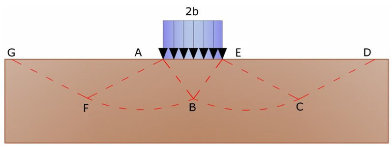
Solution of Prandtl
Once the soil tending to failure by application of the bearing capacity is identified, it can be calculated expressing the equilibrium between the forces acting in any volume of soil whose base is delimited by whichever slip surface.
Thus we reach the equation:
![]()
where the coefficient B depends only upon the soil’s angle of friction φ'. Forφ'≠0 the factor B = 5,14.
In the alternate case, namely that where the soil is cohesionless (c=0, γ'≠0) q'=0 so that according to Prandtl it would not be possible to apply any load to cohesionless soils.
This theory, even if not practically applicable, has been the base for all the following researches and computation methods.
Caquot, indeed, continued from the same premises as Prandtl excepting that the load strip is no longer placed on the surface but at a depth h, where h < 2b; the soil between surface and the depth h has the following characteristics: γ'=0, φ'≠0, c'=0 and is a material with weight attribute but with no resistance.
Solving the equilibrium equations it is possible to obtain the following expression:
![]()
which is certainly a step forward but hardly reflects reality.
Terzaghi (1955)
Terzaghi, continues on the same lines as Caquot but adds modifications to take into account of the real characteristics of the foundation-soil system.
Under the action of the load transmitted by the foundation, the soil at the contact with the foundation tends to move laterally, but is restrained in this by the tangential resistances that develop between the soil and the foundation. This results in a change of the stress state in the ground placed directly below the foundation.
Terzaghi assigns to the sides AB and EB of Prandtl’s wedge, an inclination Ψ to the horizontal, assigning to this a value as a function of the mechanical characteristics of the soil at the contact soil-foundation.
Thus γ' =0 for soil below the foundation is reviewed assuming that the failure surfaces remain unaltered, the expression for bearing capacity becomes:
![]()
where:
C is a coefficient that is a function of the angle of friction φ of the soil below the footing and of the angle φ defined above
b is the half width of the strip
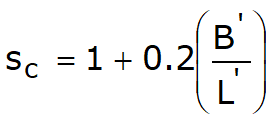
Furthermore, on the basis of experimental data, Terzaghi introduces factors due to the foundation shape.
Again Terzaghi refines the original hypothesis of Prandtl (who considered the behaviour of soil as rigid–plastic) and assigns such behaviour only to very compact soils. In these soils the loads/settlements curve is linear at firstand then becomes short curved (elastic-plastic behavior). Failure is instantaneous and the value of the bearing capacity is easily identifiable (general failure).
In a very loose soil however the relation loads/settlements has an accentuated curved line even at low levels of load due to a progressive failure of the soil (local failure) and thus the identification of bearing capacity is not so clear like for compact soils..
For very loose soils Terzaghi considers the previous formula introducing some reduced values of the soil mechanical properties:
![]()
![]()
Thus Terzaghi’s formula becomes:
![]()
where:
![]()
![]()
Foundation type: |
Strip |
Circular |
Square |
|---|---|---|---|
Sc |
1.0 |
1.3 |
1.3 |
Sg |
1.0 |
0.6 |
0.8 |
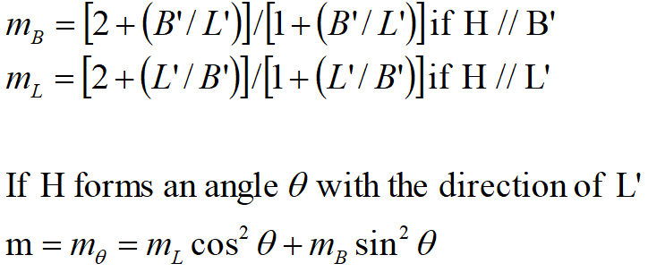
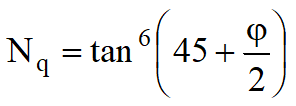
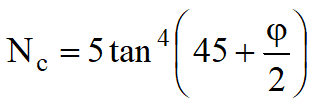
Meyerhof (1963)
Meyerhof proposed a formula for bearing-capacity calculation similar to that of Terzaghi but introduced more foundation shape factors as sq that multiplies with the depth term Nq; including furthermore, depth factors di and inclination factors ii for the cases where the load line is inclined to the vertical.
Meyerhof obtained the N factors by making trials with BD arc (see Prandtl mechanism) which include an approximation for shear along ”shallow” foundations (soil lateral support)..
The N factors are given below together with the complete formula:
|
|
![]()
![]()
![]()
Factors of
|
Value |
For |
|---|---|---|
Shape |
|
whatever j |
|
φ >10 |
|
|
φ =0 |
|
Depth |
|
whatever j |
|
φ >10 |
|
|
φ =0 |
|
Inclination
where :
θ=inclination of the resultant on the vertical |
|
whatever j |
|
φ >10 |
|
|
φ =0 |
Factors of form, depth and inclination that appear in the formula of Meyerhof
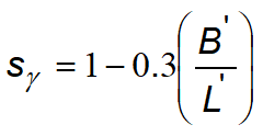
Hansen (1970)
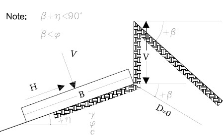
Hansen’s formula is considered like a further extension of the earlier Meyerhof equation. These extensions consist of the introduction of bi that considers the possible tilting of the footing from the horizontal and a ground factor gi for the possibility of a slope of the ground supporting the footing.
Hansen’s formula is valid for whatever ratio D/B and therefore for both shallow footings and deep bases, however the author introduces coefficients to compensate for the excessive increment in bearing capacity with the depth increasing.
Shape factors |
Depth factors |
Load inclination factors |
Soil inclination factors |
Bearing surface inclination factors |
|---|---|---|---|---|
|
|
|
|
|
|
|
|
|
|
|
|
|
|
|
|
|
|
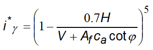
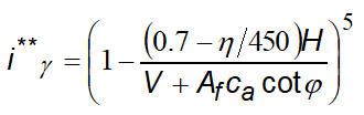
•the expressions with (') are valid when φ=0. •Af= effective area of the foundation (B' x L') •D= depth of the foundation in the soil, to be used with B and NOT with B'. •ca= the adhesion to the base, equal to the cohesion or to a fraction of it |
|
|
|
|
||
* η=0 ** η>0 *** strip foundations |
||||
Factors proposed by Hansen for the computation of qult
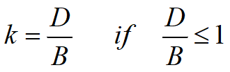
D/B |
0 |
1 |
1.1 |
2 |
5 |
10 |
20 |
100 |
d'c |
0 |
0.40 |
0.33 |
0.44 |
0.55 |
0.59 |
0.61 |
0.62 |
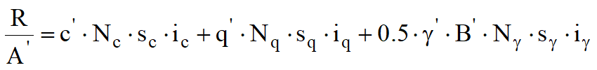
Vesic (1975)
Vesic proposes a formula that is analogous to taht of Hansen's with Nq and Nc Meyerhof's terms and Nγ as follows:
![]()
Shape and depth factors are the same than Hansen’s but there are differences in load inclination factors, ground inclination factors (foundation on slope) and bearing surface inclination factors (inclined base).
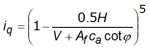
Brich-Hansen (EC 7 - EC 8)
In order that a foundation may safely sustain the design load in regard to general failure for all combinations of load relative to the ultimate limit state, the following expression must be satisfied:
![]()
where:
•Vd is the bearing capacity, normal to the footing ground, including the weight of the foundation itself
•Rd is the foundation design bearing capacity for normal loads, also considering the eccentric and inclined loads
To better estimate Rd for fine grained soils short and long term situations should be considered. Bearing capacity in drained conditions is calculated by:

where
|
Design effective foundation area. Where eccentric loads are involved, use the reduced area at whose center the load is applied. |
cu |
Undrained cohesion.
|
q |
Total lithostatic pressure on bearing surface
|
|
Shape factor for rectangular foundations |
|
Shape factor for square or circular foundations |
|
Correction factor for the inclination due to a load H |
|
Correction factor that takes into account the inclination of the base of the foundation |
Design bearing capacity in drained conditions is calculated as follows:
where:
|
|
|
Shape factors |
Resultant inclination factors due to a horizontal load H |
||
|---|---|---|---|
|
rectangular |
|
|
|
square or circular |
|
|
|
rectangular |
|
|
|
rectangular, square or circular |
||

Correction factors proposed by Brinch-Hansen for the computation of qult
In addition to the correction factors reported in the table above will also be considered the ones complementary to the depth of the bearing surface and to the inclination of the bearing surface and ground surface (Hansen).
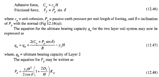
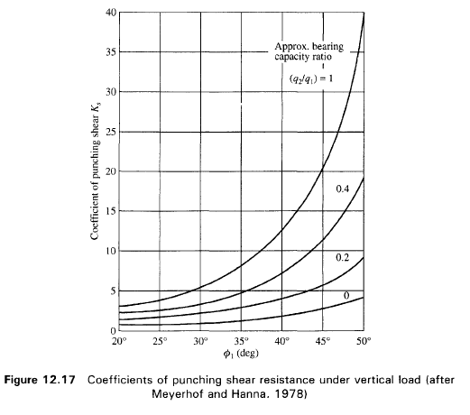
Meyerhof e Hanna (1978)
All the theoretical analysis about bearing-capacity calculation are based on the assumption that the soil is isotropic and homogeneous to a considerable depth but in nature, soil is generally non-homogeneous and it can be constituted by different percentages of granulometric component such as gravel, sand, silt and clay. However, the assumption of homogeneity to such soils is not strictly valid if the failure surface cuts across boundaries of distinct layers with different strength characteristics and compositions.
The present analysis is limited to a system of two distinct soil layers. For a footing located in the upper layer at a depth D, below the ground level, the failure surfaces of bearing capacity can develop on the upper layer or also involve the second layer. The condition that the upper layer is stronger than the lowest is possible and vice-versa. In both cases, a general analysis with c = 0 will be presented and will be valid also for sand or clay.
The bearing capacity of a layered system was first analyzed by Button (1953) who considered only saturated clay (φ = 0). Later on Brown and Meyerhof (1969) showed that the analysis of Button leads to unsafe results. Vesic (1975) analyzed the test results of Brown and Meyerhof and others and gave his own solution to the problem.
Vesic considered both the types of soil in each layer, that is clay and (c = 0) soils. However, confirmations of the validity of the analysis of Vesic and others are not available. Meyerhof (1974) analyzed the two layer system consisting of dense sand on soft clay and loose sand on stiff clay and supported his analysis with some model tests.
Again Meyerhof and Hanna (1978) advanced the earlier analysis of Meyerhof (1974) to encompass (c = 0) soil and supported their analysis with model tests. The present section deals briefly with the analyses of Meyerhof (1974) and Meyerhof and Hanna (1978).
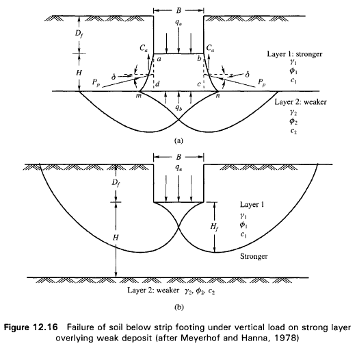
Case 1: A Stronger Layer Overlying a Weaker Deposit
Figure 12.16(a) shows a footing at a depth D with a width B , in a strong soil layer (Layer 1). The depth to the boundary of the weak layer (Layer 2) below the base of the footing is H. If this depth H is insufficient to form a full failure plastic zone in Layer 1 under the bearing capacity conditions, a part of this bearing capacity will be transferred to the boundary level mn. This load will induce a failure condition in the weaker layer (Layer 2). However, if the depth H is relatively large then the failure surface will be completely located in Layer 1 as shown in Fig. 12.16b.
The ultimate bearing capacities of strip footings on the surfaces of homogeneous thick beds of Layer 1 and Layer 2 may be expressed as follows:
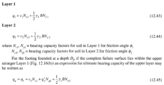
If q1 is greater than q2 and if the depth H is insufficient to form a full failure plastic condition in Layer 1, then the failure of the footing is due to the earth pressure of soil that develops from the weakest layer toward the strongest layer. The resisting force for punching may be assumed to develop on the faces ad and be passing through the edges of the footing. The forces that act on these surfaces are (per unit length of footing),
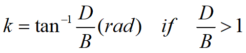
Richards, Helm and Budhu (1993) developed a procedure that allows, under seismic conditions, to evaluate both the bearing capacity and induced settlements, therefore to proceed to the verification of both limit states (ultimate and damage). In this case, the calculation of the bearing capacity is performed considering the presence of inertial forces in the foundation soil due to earthquake, while the computation of settlements is obtained through an approach Newmark type. The authors have extended the classical formula of the bearing capacity as follows:
![]()
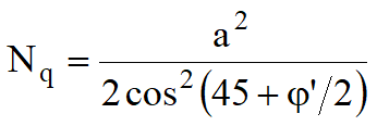
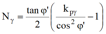
Where the bearing capacity factors are calculated using the following formulas:
![]()
![]()
![]()
The authors, furthermore, examined a mechanism type Coulomb with the limit equilibrium approach, considering also the acting inertia forces on the failure terrain volume . In the static field, the classical Prandtl mechanism may be approximated as shown in the figure below, removing the transition zone (range of Prandtl) considering onlythe line AC, which is considerated as an ideal wall in equilibrium under the action of active and passive thrust that it receives from I and III wedges:
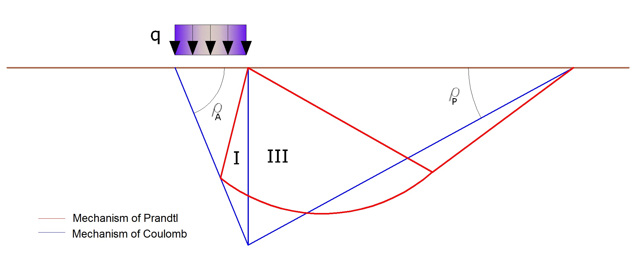
Computation of bearing capacity qlim
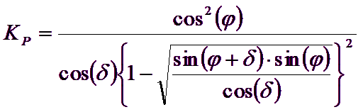
The authors have obtained the: i) the expressions of ρA and ρP angles that define the areas of active and passive thrust and ii) the active and passive thrust coefficients KA and KP as a function of the angle of internal friction φ of the ground and the angle of friction d ground - ideal wall:
![]()
![]()

It is possible to observe that the use of previous equations assuming φ = 0.5δ, leads to the value of the bearing capacity factors very close to those based on an analysis of Prandtl. Richards et. al (1993) used the Coulomb mechanism in seismic case, taking into account the inertia forces acting on the ground volume in failure. These mass forces, due to acceleration kh g and kv g, respectively acting in horizontal and vertical direction, are equal to kh g and kv g. Were thus obtained the extensions of the expressions of ρA and ρP, as well as KA and KP, respectively indicated as ρAE and ρPE, and KAE and KPE to denote the seismic conditions:
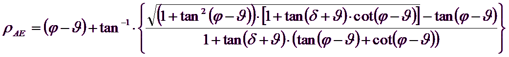
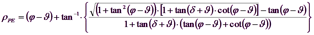

The values of Nq and Nγ can also be determined using the above formulas, of course, using the expressions of the ρA and ρP angles and of KAE and KPE coefficients related to the seismic case. In these expressions appears the angle θ defined as:
![]()
The table below shows the bearing capacity factors calculated for the following parameter values:
φ = 30°
δ = 15°
And for several values of the seismic thrust coefficients:
kh/(1-kv) |
Nq |
Ng |
Nc |
|---|---|---|---|
0 |
16.51037 |
23.75643 |
26.86476 |
0.087 |
13.11944 |
15.88906 |
20.9915 |
0.176 |
9.851541 |
9.465466 |
15.33132 |
0.268 |
7.297657 |
5.357472 |
10.90786 |
0.364 |
5.122904 |
2.604404 |
7.141079 |
0.466 |
3.216145 |
0.879102 |
3.838476 |
0.577 |
1.066982 |
1.103E-03 |
0.1160159 |
Table of bearing capacity factors for φ=30°
Bearing capacity for foundations on rock
Where foundations rest on rock, it is appropriate to take into consideration certain other significant parameters such as the geologic characteristics, type of rock and its quality measured as RQD. It is the practice to use very high values of safety factor for bearing capacity of rock and correlated in some way with the value of RQD (Rock quality designator). For example for a rock whose RQD is up to a maximum of 0.75 the safety factor oscillates between 6 and 10. Terzaghi’s formula can be used in calculation of rock bearing capacity using friction angle and cohesion of the rock or those proposed by Stagg and Zienkiewicz (1968) according to which the coefficients of the bearing capacity are:
|
|
|
These coefficients should be used with form factors from the formula of Terzaghi. Ultimate bearing capacity is a function of RQD as follows:
![]()
If rock coring does not render whole pieces (RQD tends to 0) the rock is treated as a soil estimating as best the factors: c and φ.
Sliding check
The stability of a foundation should be verified with reference to collapse due to sliding as well as to general failure. For collapse due to sliding, the resistance is calculated as the sum of the adhesion component and the soil-foundation friction component. Lateral resistance arising from passive thrust of the soil can be taken into account using a percentage supplied by the user.Resistance due to friction and adhesion is calculated with the expression:
![]()
where
| Nsd | is the value of the vertical force |
| δ | is the angle of shearing resistance at the base of the foundation |
| ca | is the foundation-soil adhesion |
| A' | is the effective foundation area; where eccentric loads are involved, use the reduced area at whose center the load is applied |
Computation of settlements
The application of a load of finite size on a cohesive soil generates a series of phenomena which can be summarized as illustrated in image below:
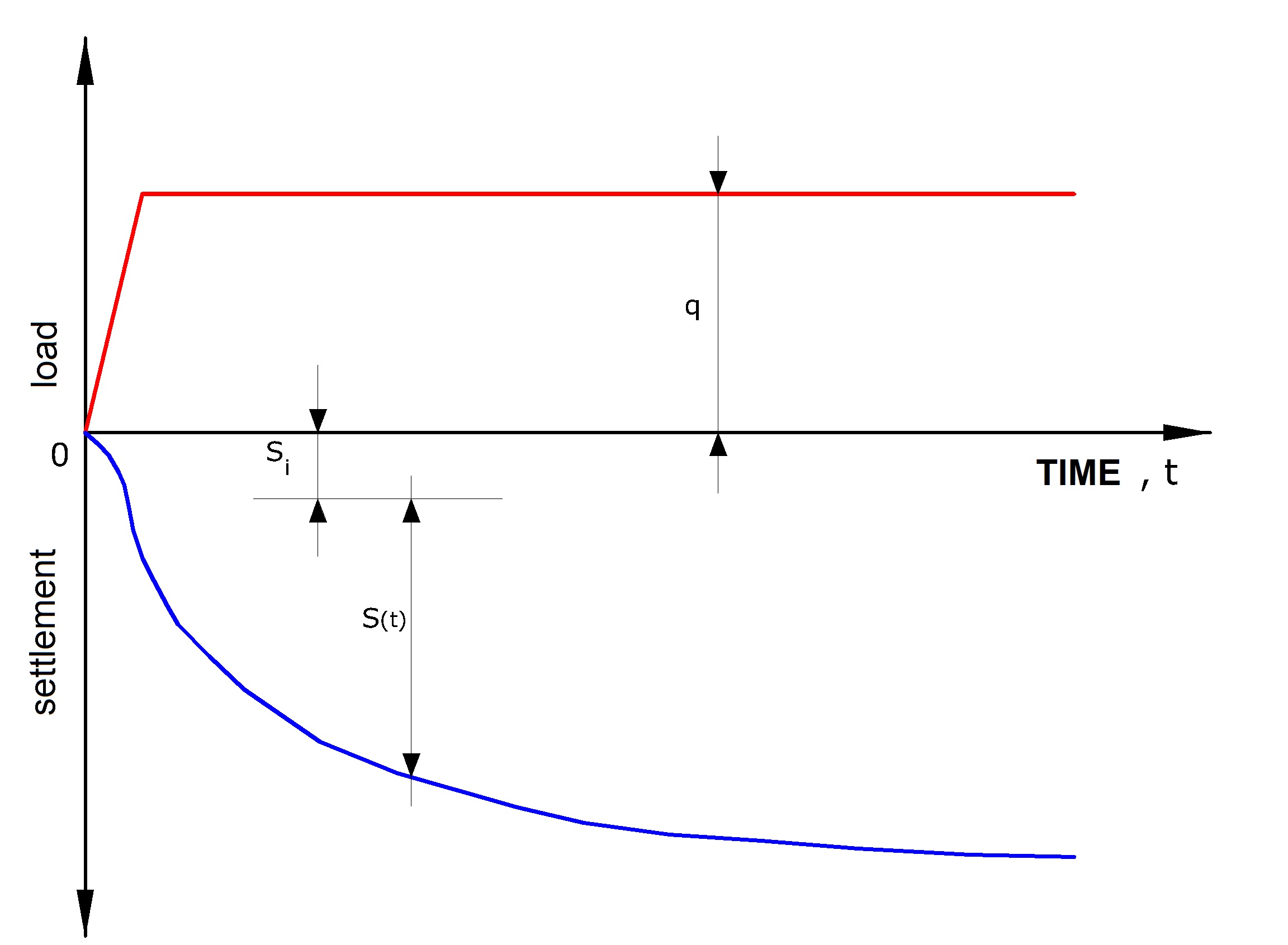
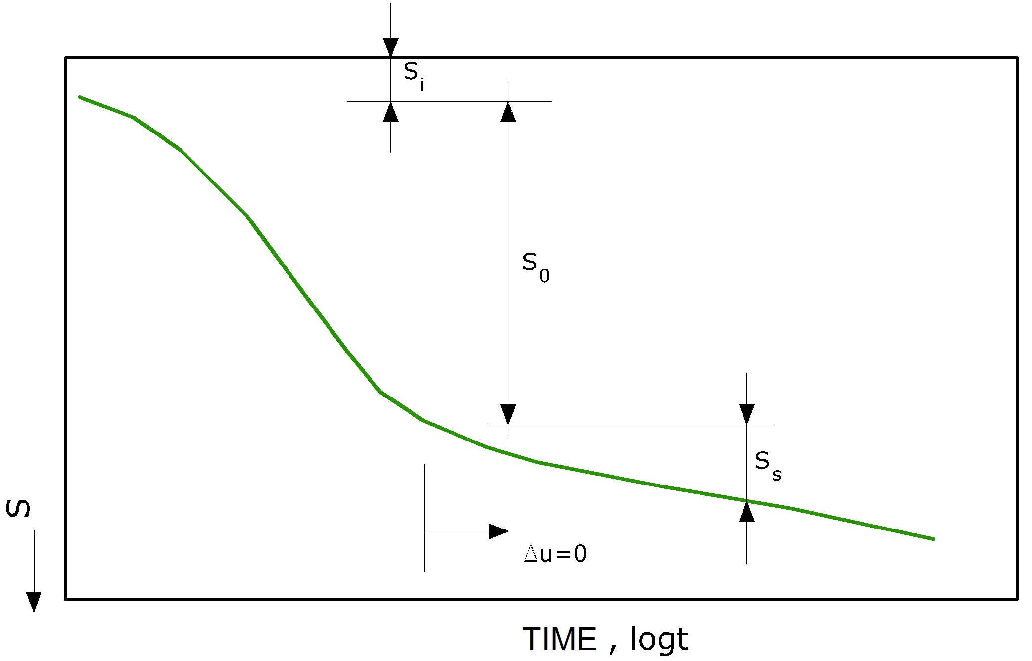
Settlement types
1.During the loading phase in the ground develop of the overpressures of interstitial water Δu, and due to the low permeability of the soil is permissible to assume that, in the context of the usual speed of application of the load, there are undrained conditions. The clay layer deforms in volume almost constant and the settlement that follows is indicated as immediate settlement.
2.The establishment of drainage, with the progressive transfer of load from the fluid phase to the solid skeleton, implies further settlements, the speed of which in time is primarily related to the drainage conditions. The process is known as primary consolidation, the analysis is conducted with the various models of the theory of consolidation. The settlement that follows in this process of expulsion of water from the interstitial voids is indicated as consolidation settlement.
3.Finally, even when the interstitial surcharges are dissipated (Δu = 0), there continue to be settling in time due to creep in drained conditions, and the settlement is known as secondary settlement.
The settlement of a rectangular foundation of size B' × L' placed on the surface of an elastic support may be calculated by use of an equation based on the elasticity theory (Timoshenko and Goodier (1951)):
![]() (1)
(1)
where:
q0 Intensity of contact pressure.
B' Minimum size of reactant area.
Es and ν Elasticity parameters for soil.
Ii =f(L'/B', H, ν, D) Influence factors that depend on: L'/B', thickness of layer H, Poisson's ratio m, bearing surface depth D
IF influence factor
Coefficients I1 & I2 may be calculated using the equations of Steinbrenner (1934) (Bowles), as functions of the relation M=L'/B' and N=H/B, using B'=B/2 e L'=L/2 for coefficients relative to the center and B'=B & L'=L for coefficients Ii at the edge.
Influence factor IF is due to Fox (1948), and suggests that settlement is reduced with depth, depending on Poisson’s ratio m, and of the ratio L/B.
In order to simplify the equation (1) the coefficient IS is introduced:

Relationship (1) can be written as:
The equation can be applied to flexible or rigid foundations with appropriate changes in the value of Is.
The author, analyzing a number of cases, has concluded that the equation formulated previously, in order to to provide good results must, be applied as follows:
1.Make the best estimate of q0
2.Convert the foundation, if circular, in an equivalent square foundation
3.Determine the point where to calculate the settlement and divide the support base so that the point is in correspondence with one of the outer edge or an inner edge common to more rectangles
4.The thickness H of the layer responsible for the settlement should be taken as the minimum of the two following values: depth z = 5B where B is the minimum overall size of the base of the foundation; depth at which is located a hard layer (ES of the layer must be about 10 times the value of the adjacent thickness).
5.Correctly calculate the ratio H/B'. For a layer thickness H=z=5B we find, for the center of the foundation, H/B'=5B/0,5B=10B, for a point 5B/B=5
6.Obtain Is having an accurate calculation of m and obtaining the influence coefficients I1 and I2 from the table proposed by the same author
7.Obtain IF with the help of the image below
8.Obtain ES in the thickness of the layer z=H as weighted average of the values of ESI of single layers in the thickness HI
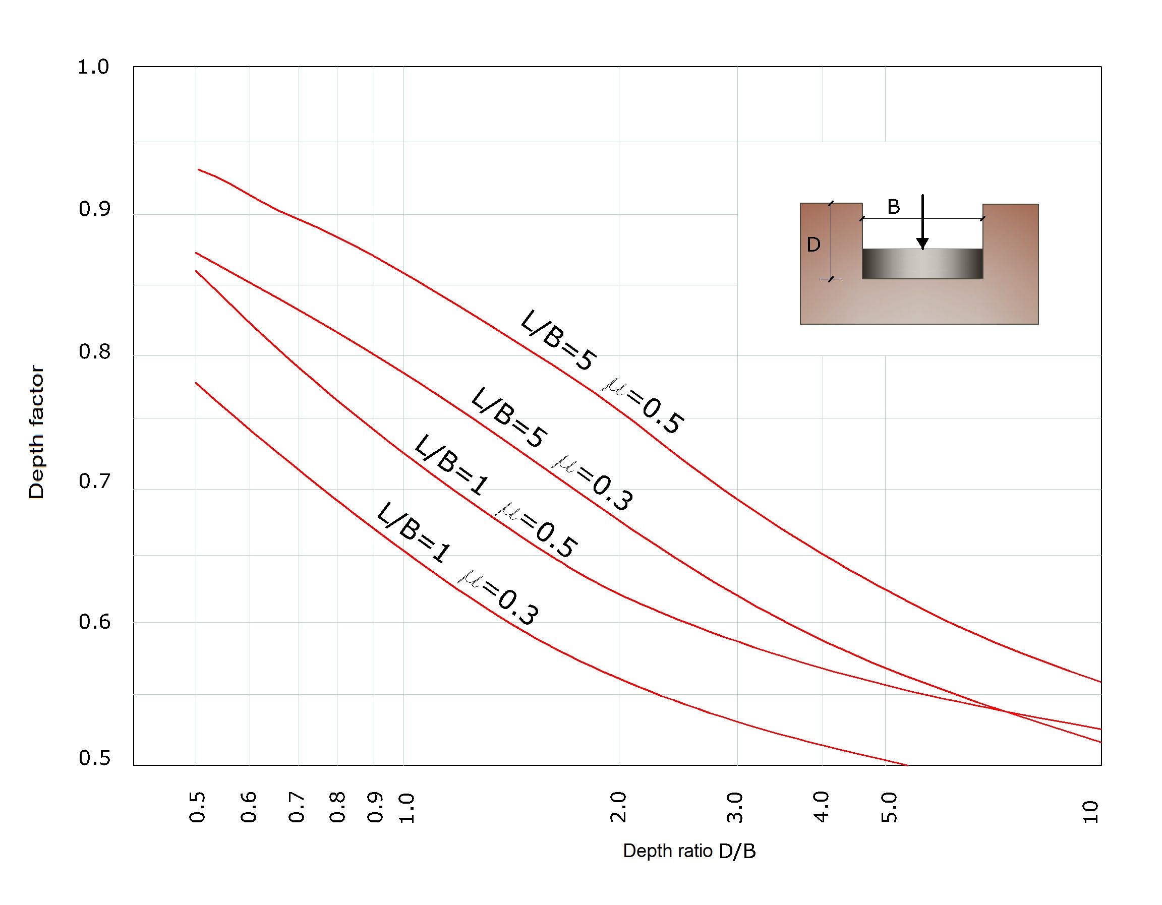
Influence factor IF for a foundation calculated at a depth D
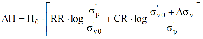
The computation of settlement with the oerdometric approach allows the evaluation of monodimensional settlement (Terzaghi-1943), produced by stresses induced by the application of a load in conditions of inhibited lateral expansion. However the computation with this method is to be considered empiric rather than theoretic. Nonetheless the ease of use and of controlling the influence of the various parameters involved make of this a very widespread method.With reference to the image below the settlement ΔH of a layer of an initial thickness H0 is given by:
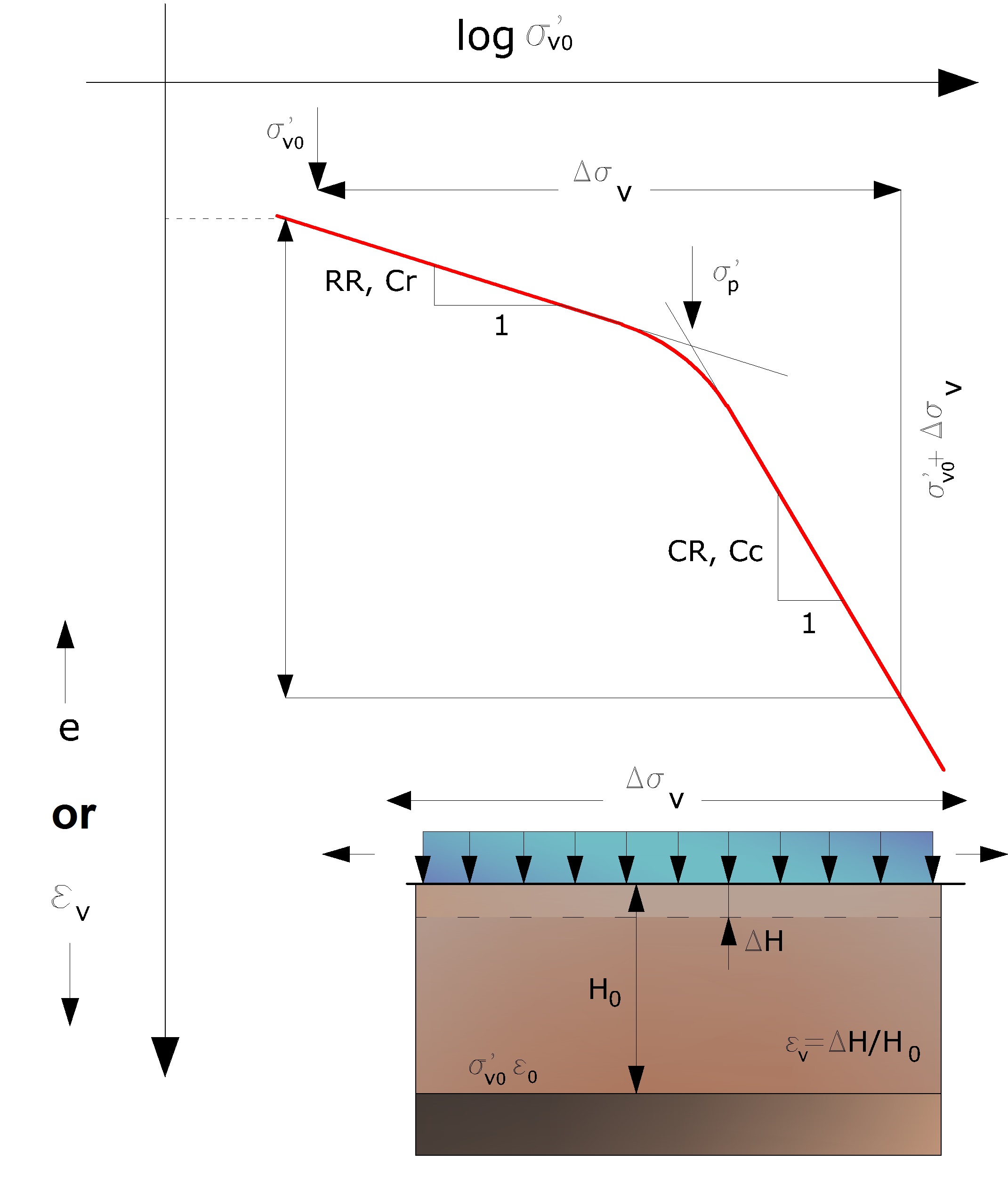
Oedometric settlement
The process of settlement calculation goes through two phases:
1.Calculation of vertical stresses induced at various depths applying the theory of elasticity (Boussinesq, Westergaard, etc.)
2.Evaluation of compression parameters through an oedometric test
With reference to the results of the oedometer test, the settlement is evaluated as:
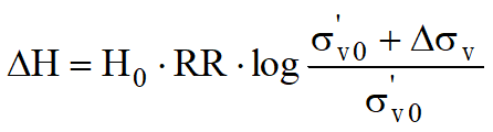
If the soil is overconsolidated (OCR>1), that is if the increment of stresses due to the application of load does not cause preconsolidation pressure to exceed σ'p (σ'v0 + Δσv < σ'p)
If on the other hand the soil is normally consolidated (σ'v0=σ'p), deformation occurs in the compression interval and the settlement is calculated as:
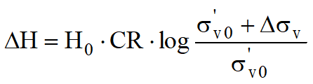
where:
| RR | Recompression ratio |
| CR | Compression ratio |
| H0 | Initial layer thickness |
| σ'v0 | Effective vertical stress before the application of the load |
| Δσv | Increment in vertical stress due to the application of the load |
As an alternative to parameters RR and CR one can refer to the oedometric modulus M, however, in such case, it will be necessary to use judgment in selecting the value to use taking account the stress interval (σ'v0+ Δσv) significant for the problem in question.
The correct application of this approach requires:
•Subdivision of compressible layers into smaller ones (max. 2.00m)
•An estimate of the oedometric modulus for each layer
•Computation of settlement as a sum of the contribution of each subdivision of small layers
Many use the formulas above to calculate settlement both for clays and sands with fine to medium granularity as the elasticity modulus is derived directly from consolidation tests. However for soils with a coarser grain, the dimensions of oedometric testers are not very significant for the global behaviour of the layer and for sands it is advisable to use penetration tests either static or dynamic.
Secondary settlement
Secondary settlement is calculated by the expression:
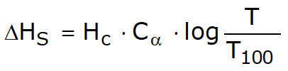
where:
| Hc | is the height of the layer in phase of consolidation; |
| Ca | is the coefficient of secondary consolidation as vector of the secondary portion of the curve Settlement-logarith time; |
| T | time for which the settlement is required; |
| T100 | time for the completion of primary settlement. |
The assumptions at the base of this method are:
•the secondary consolidation starts after the exhaustion of the primary consolidation process;
•the value of Ca can be considered constant during the evolution of the secondary settlement.
Schmertmann settlements
Schmertmann (1970) proposed an alternative method of calculating settlement as related to the variation to the pressure bulb on deformation.
Thus Schmertmann proposes a triangular deformation diagram where the depth at which significant deformation occurs is 4B for strip foundations and 2B for square or circular foundations.
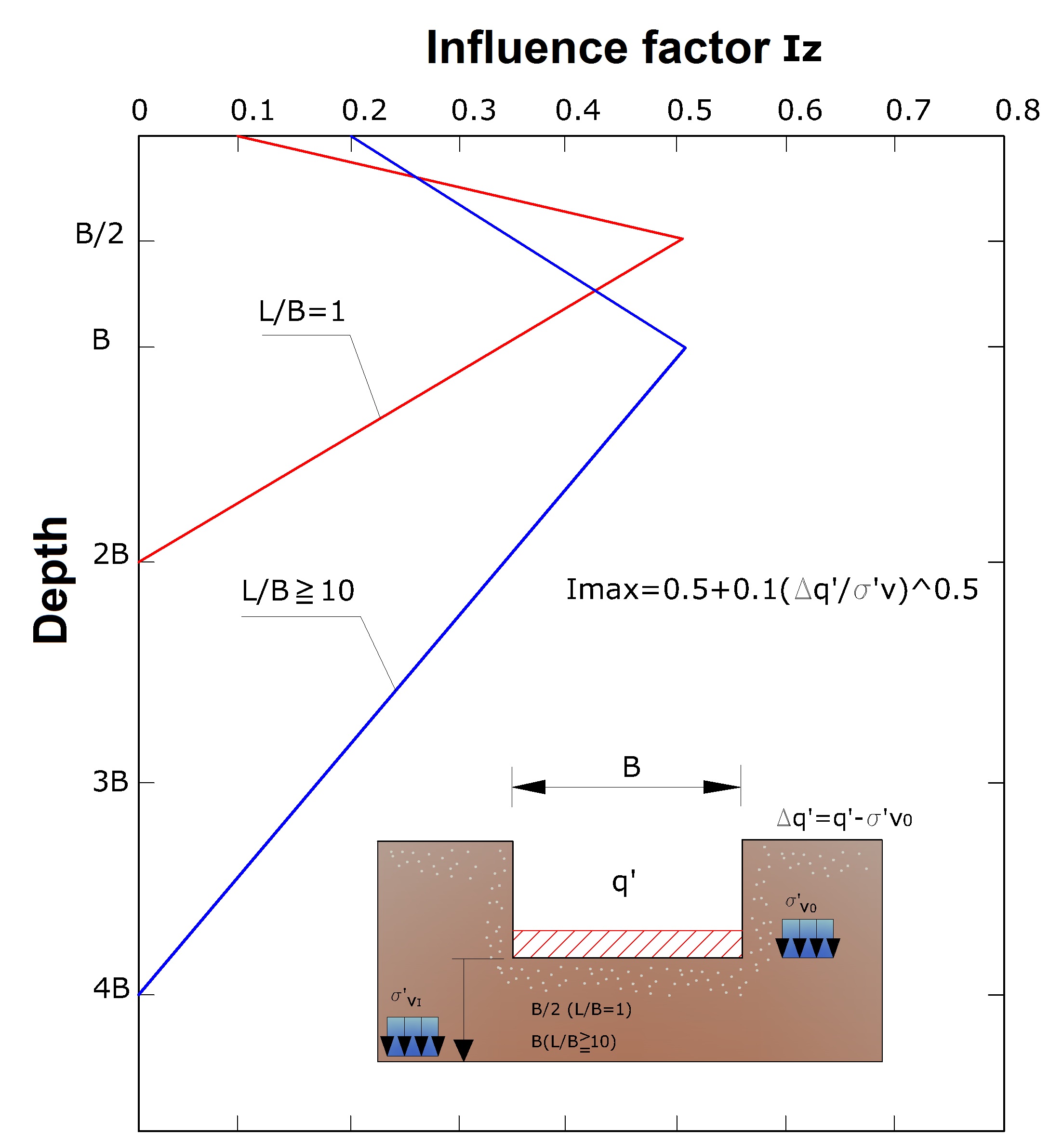
Variation of the influence factor with depth
With this approach settlement is expressed by the following expression:
![]()
Where:
Δq is the net load applied to the foundation;
Iz is a deformation factor whose value is null at depth 4B or 2B respectively for Strip or Round/Square foundations.
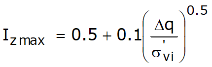
Where:
σ'v0 is the effective vertical stress at depths of B/2 for round or square foundations and at depth B for strip foundations
Ei is the modulus of soil deformation corresponding to the i-th layer considered in the calculation;
Δz is the thickness of the i-th layer;
C1 and C2 are two correction factors.
Modulus Ei is assumed as 2.5 qc for square/round foundations and 3.5 qc for strip foundations. For intermediate cases the value is interpolated dependent on the value of L/B.
The term qc in the determination of Ei is the CPT tip resistance.The expressions for C1 and C2 are:
|
That accounts for footing depth |
|
That accounts for the deformations, different in time, due to secondary effect |

Where t represents the time in years, after completion of the structure, for which settlement is calculated.
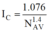
Burland and Burbidge settlements
There where dynamic penetration test results are available, it is possible to rely on Burland and Burbidge (1985) method for settlement computation for which an index of compressibility Ic is correlated to the result NSPT of the dynamic penetration test. The formula proposed by the authors is:

Where:
q' gross effective pressure;
σ'v0 effective vertical stress at footing depth;
B width of the foundation;
Ic compressibility index;
| fs, fH, ft | corrective factors that account respectively for the form, compressible layer thickness and time, for the viscous component |
Ic, compressibility index is related to the average value NAV of NSPT at a significant depth zi:
To calculate the value of zi it is used the following relationship:
![]()
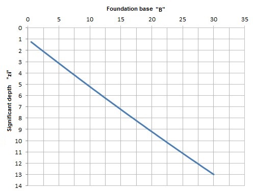
Trend of the significant depth as a function of the foundation base
As regards the NSPT values to use in calculating the average NAV, it is opportune to remember that values should be corrected for sands with silt content under the water table and NSPT >15 as indicated by Terzaghi & Peck (1948):
![]()
Where Nc is the corrected value to use in calculation.
For gravel or gravelly sandy deposits, the corrected value is:
![]()
For corrective factors fS, fH ed ft the expressions are:
|
|
|


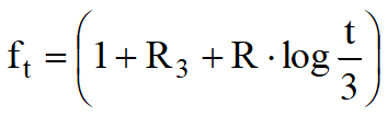
Where
t = time in years > 3;
R3 = a constant of value 0.3 for static loads and 0.7 for dynamic loads;
R = a constant of value 0.2 for static loads and 0.8 for dynamic loads.
|
© GeoStru