The term filtration indicates that physical phenomenon for which occurs the passage of water from an area with a given energy to other area with a lower energy, through a porous medium. The energy can be expressed as the sum of kinetic energy related to the velocity of the fluid, of the potential energy depending on the position of the point and of the pressure of the liquid at the same point. Since the rate of filtration is always very small the kinetic term is negligible. In studying the filtration of water can appear problems, both of permanent and unsteady motion flow. With reference to the pressure of water, which plays an important role in most of the stability problems, please note that in permanent motion it remains constant over time, while in unsteady flow is a function of time and it may rise or fall.
With reference to the amount of water in the phenomenon of filtration through a certain area, please note that in continuous operation the amount of' water that enters is equal to that coming out, while under unsteady flow there is no equality and the difference represents the volume of water that is accumulated or expelled from the ground in the time interval considered. In the phenomenon of consolidation, which is a particular condition of unsteady flow, also interferes the compressibility of the soil. In steady state the area in which filtration develops, in the scheme of representation that is adopted, has two types of boundaries: one is the place where is known the water load and defines the border or boundary condition of the potential; the other one is an outline of waterproof materials, such as impermeable rock, clay, etc. which delimits the layer in which the filtration occurs and is defined as border or boundary condition of the water flow. To clarify what was said just remember for example the conditions of water flow in the constant load permeability test. In this test clearly the boundaries of the potential are the surfaces of the entry and exit of water from the soil sample. Because the container walls are impermeable, the flow is parallel to the container and the wall forms the boundary of the water flow:
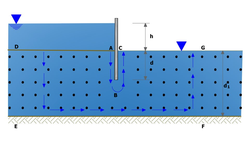
Scheme for the water flow
A practical case is the sheet piling (previous figure) that maintains a constant level h of water and which is driven into the soil to a depth d in a homogeneous layer of permeable soil (sand or gravel) of thickness dI, which rests on a impermeable layer (rock or clay). In this case we are talking about a confined flow, since the boundary conditions of the region in which the motion takes place are geometrically defined. The water flow is caused by the hydraulic load h; on the surface AD acts a constant load and this surface is the first boundary of the potential in our problem; on CG the load is also constant and this constitutes the second boundary. Obviously, to fulfill its task, the sheet piling must be impermeable, so its surface ABC is one of the boundaries of the flow while the surface EF of the impermeable layer will form the other border. Obviously in principle if the characteristics of water, soil and the impermeable layer, upstream and downstream of the sheet piling, are constant it can be considered that the points D, E, F and G are endlessly; in practice it is generally considered that the length concerned is included within 4-5 times the thickness of the layer. To determine the amount of water that seeps into the ground will make the assumption that the water flow is governed by Darcy's law and that the soil is homogeneous, isotropic and incompressible:
![]()
Darcy's law is valid for laminar flow, a condition that occurs for certain values of the Reynolds number, R. The value of R, that characterizes the flow passing from laminar to turbulent, takes different values depending on the authors; Taylor (1948) has indicated as a criterion for the validity of Darcy's law R <= 1. Other researchers have examined, especially for clay, the connection between the flow conditions and the hydraulic gradient; in particular Tavenas ed al. (1983) have come to the conclusion that, with regard to the clays, the Darcy's law is valid for gradients between 0.1 and 50.
To calculate the flow rate of filtration through the soil it is useful to determine the distribution the pore water pressure via the construction of the flow grid, that is, the system of streamlines and equipotential lines representing the flow of water through an incompressible soil. Accepting the hypothesis of incompressible ground for filtration motion in plane and steady conditions the continuity equation can be written in the form:
![]()
The two components of the velocity of the liquid, according to Darcy's law, can be expressed in the form:
![]()
![]()
Combining these three equations is obtained:
![]()
which is the Laplace equation for permanent motion on a plane, on the assumption of homogeneous, isotropic and incompressible material. This equation can be expressed by means of two conjugate functions φ and ψ. Indeed, we can express the velocity components as partial derivatives with respect to x and z of the function φ = k h :
![]()
![]()
Then we can also write:
![]()
The existence of the function φ = k h, according to velocity potential for a fluid in motion, implies null vorticity and that the motion is irrotational. We can then say that it is a function of stream such that:
![]()
So we have:
![]()
![]()
And we can also write:
![]()
φ and ψ are known, respectively, as a function of potential and function of stream. Taking up the case before indicated, the water that seeps through the soil at the bottom of a pile wall (figure below) we notice that two equipotential lines are the surfaces of the upstream and downstream ground of the same sheet piling; Furthermore the surface of the impermeable layer is a stream line or a flow line. By solving the Laplace equation in accordance with these boundary conditions, we can construct the flow net. Each strip between two adjacent flow lines is a flow channel and each part of the flow channel comprised between two equipotential lines is a field. It is therefore convenient to build the equipotential lines in a manner that the piezometric height difference between two successive lines is constant and the flow lines in such a way that each flow channel has a constant flow. If h is the total hydraulic load and Na is the total number of identified piezometric height differences, the difference in hydraulic load between two successive equipotential lines is:
![]()
In a point z as shown in the following figure the pressure is:
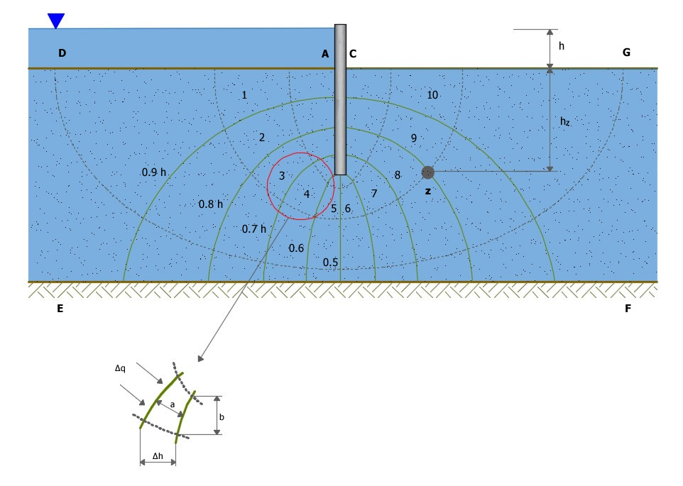
Schematization of the flow net
Being n the number of piezometric height differences crossed to arrive in z, in the example on the previous figure we have:
![]()
If there were no flow of water, that is, if the downstream surface were impermeable, the hydrostatic pressure at this point would be:
![]()
since the water moves, there is a loss of load which according to the filtration net drawn at the point z is equal to 8/10h. The excess water pressure at the point z is then given by:
![]()
To know the extent of filtration flow we consider a field, that is, an area between two flow lines and two equipotential lines; the length of the side in the direction of the flow lines is a and therefore the hydraulic gradient in a field is:
![]()
and the velocity:
![]()
Assuming that the other side of the field is of length b, then the flow through the field per length unit of sheet piling will be:
![]()
for each flow tube; if b = a, that is, if the elements of the filtration net are square, we get:
![]()
If Nb is the total number of flow channels of the total flow per length unit of sheet piling will be:
![]()
In this way, when it is constructed the flow net, one can easily calculate the flow rate. The filtration net is often built with experimental methods in the laboratory, with analog models graphically or by trial. In complex situations of the subsoil, for succession of layers and anisotropy of permeability, one can get the filtration net by means of numerical methods (FEM, BEM, finite difference method).
© GeoStru