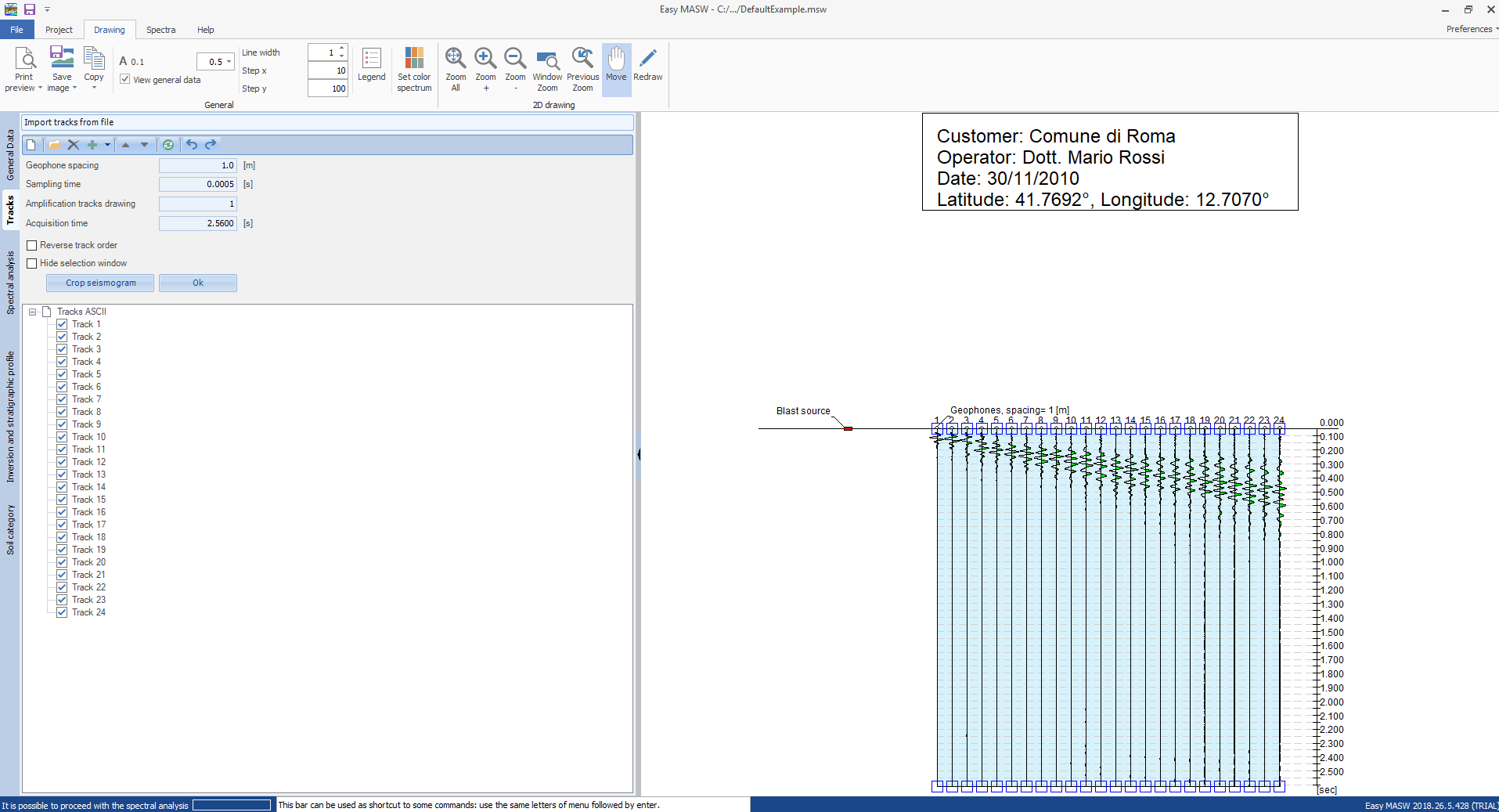
In this section the data to process is imported into the program. It is possible to import tracks from standard files SEG-2 (both with the extension. Sg2 and Dat) or from text files.
It is possible to import multiple tracks in the same project and shift their order depending on the needs. If necessary you can also automatically reverse the order of the tracks using the appropriate option. The import of multiple files can be done by:
•inserting the new tracks in the queue of existing ones;
•inserting the new tracks before the existing ones;
•interposing the new tracks among the existing ones.
If you are importing tracks from a SEG2 file, in the control list on the left side of the window you can find all information recorded by the instrument in acquisition phase including the sampling time.
To import the tracks from one or more text files it is necessary that the data contained to follow a convention. If each file contains a single track, it should consist of lines each of which has the datum associated with the acquired sample. If a file contains more tracks, they must be organized in columns in which the default separator is the character ";". It is possible to set a different character to consider as tracks separator using the appropriate summary window that appears after opening the file.
Once the import of the tracks was concluded and they were represented on the diagram, you can select the tracks to exclude from the computation acting on the control list on the left side of the screen. You can also limit the acquisition time and find the useful part of the acquired signals to cut the tracks to analyze. To perform a cut, just select the useful part of the track directly on the diagram and confirm the selection by pressing the Ok button. The cut is applied to the area selected using a logarithmic law of decay that extends to a maximum of 20 samples.
The buttons "Cancel" and "Restore" in the toolbar of the selection panel on the left, allow to operate with more flexibility.
To perform the computation you must set the spacing of the geophones and the sampling period of the tracks. If the tracks were imported from a SEG-2 file, the sampling period is automatically determined and set by the program.
Other operations that can be made at this phase are:
•export the displayed image;
•fit the size of texts;
•operate on the graph with tools such as zoom, pan etc.
Offset
By offset we are referring to the distance between the energization point and the first geophone of the same seismic. Even though its position is represented graphically, the offset does not affect the interpretation and for such reason, in Easy Masw, it is not required in the input fields. In other words, varying the offset does not alter the spectrum.
The offset is very important in the signal acquisition phase: acquisitions with different offsets on the same seismic line provide more-or-less different spectrums, depending on the lithological complexity between the beating point and the last geophone inserted on the seismic line.
In principle, it can be said that by increasing the offset we lose information on the first layer for the benefit of the deeper ones. If the offset and the stringing are low (< 40-50m) we risk losing information in depth, during acquisition phase.
Multiple experiments for this case (offset proximity to first geophone) demonstrated the presence of signal disturbances due to overlapping of P, S and R waves.
It is advisable to achieve acquisitions with “minimum offset”. We usually adopt the formula:
offset= (3-4 volte) x interdistanza dei geofoni (non minore di 4 m)
It is also recommended to carry out acquisitions by varying the offset from the minimum to a distance equal to half of the stringing. The processing of the signals acquired by varying the offset provides a better general representation to portray.
The data that the user must provide as input to the program are:
-intergeophonic distance (m): the default being 1m;
-sampling period (s): usually read from the acquisition file (0.001s order of magnitude);
-acquisition time (s): read from the acquisition file (approximately 2.0480s).
-
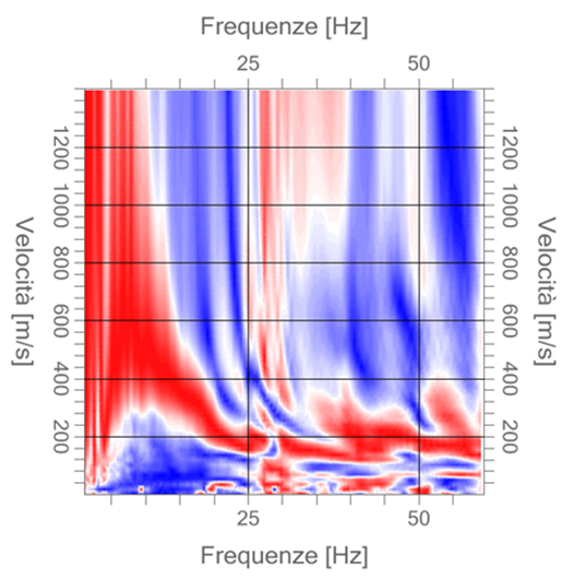
The following image represents the frequency-velocity spectrum of an acquisition:
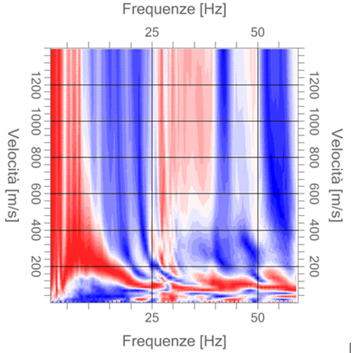
By vividly examining the above image, we can see a variation in passing bands between the maximum area (red) and the minimum area (blue), due to the number of layers the software uses to draw the spectrum, which by default is 20.
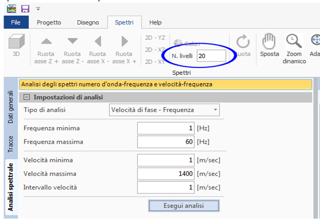
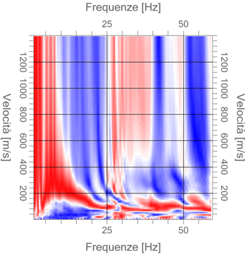
If the number of levels is set to 60, we obtain a more shaded spectrum. The layer number variation only produces a graphical effect and does not affect the computation.
In order to demonstrate the above, we follow with the same process done by a different software that allows to vary the offset position.
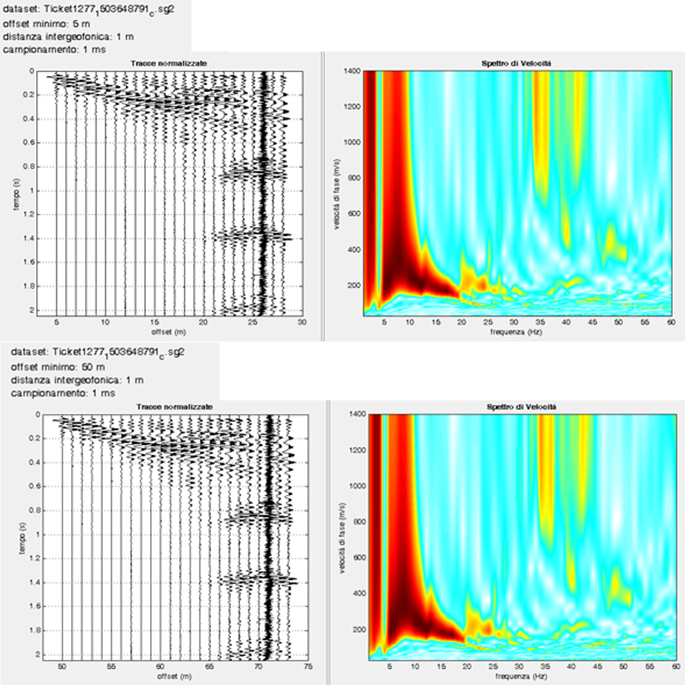
By varying the offset from 5 to 50 meters, the spectrum does not change. The only difference between the outputs of the two software is graphical. By comparison, Easy Masw provides a very well-defined spectrum, even in case of high frequencies.
The data that must not be modified is the following: intergeophonic distance, sampling period, acquisition time. Manipulating this data will distort the interpretation.
The following image shows how varying the intergeophonic distance from 1 meter (acquisition parameter) to 2 meters (inserted by the user in Easy Masw) affects the spectrum. This parameter affects the computation.
© Geostru