The probability
Probability theory is the mathematical study of probability.
Mathematicians refer to the probabilities as numbers in the range from 0 to 1, assigned to "events" whose occurrence is random.
The probability is a number associated with an event (resulting from the observation of an experiment) that may or may not occur.
A priori classical probability
If N is the total number of cases of the sample space of a random variable and n is the number of favorable cases for which the event A is realized, the a priori probability of A is given by:
![]()
The a priori probability can assume a value between 0 and 1. A probability equal to 0 indicates that the event is impossible, a probability equal to 1 indicates that the event is certain.
Frequentist probability
If m is the number of trials in which the event A occurred at a total of M trials, the probability of A is given by:
![]()
The limit that appears in this definition should not be understood in a mathematical sense, but in an experimental way: the true value of the probability is found only by making an infinite number of trials.
Indicators of a statistical distribution
The description of the data from a statistical sample is done by determining the distribution of the relative frequencies, which implicitly contains all the information that can be drawn from the sample.
The indicators are parameters that describe quantitatively the general aspects of the statistical distribution.
•In the probability theory the probability or distribution function of a discrete random variable x is a function of a real variable that assigns to each possible value of x the probability of the event.
•The expected value m (also called average or hope) of a random real variable x is a number that formalizes the heuristic idea of average value of a random phenomenon and is defined as:
•The variance of a random variable x is a number Var(x), which provides a measure of how different are the values taken by the variable, ie how much they deviate from the mean m. The variance of x is defined as the expected value of the square of the random centered variable. In statistics is often preferred the square root of the variance of x, the standard deviation indicated by the letter σ. For this reason, the variance is indicated with σ2. In statistics are used usually two estimators for the variance of a sample of cardinality n:
 e
e 
The estimator sn-1 has an expected value equal to its variance, by contrast, the estimator sn has a value different from the expected variance. A justification of the term n-1 is given by the need to estimate also the mean. If the mean μ is known, the estimator sn becomes correct.
•Starting from the standard deviation is also defined the coefficient of variation or relative standard deviation as the ratio between the standard deviation and the arithmetic mean of the values:
![]()
This new parameter (often used as a percentage) is used to make comparisons between different types data dispersions, regardless of their absolute amounts.
The way in which is distributed the probability of a random variable depends on many factors, and, as there are infinite possible graphics of functions, we can have endless ways for different probability distributions.
The most significant probability distributions are:
1) Normal distribution
2) Lognormal distribution
3) Student's t-distribution
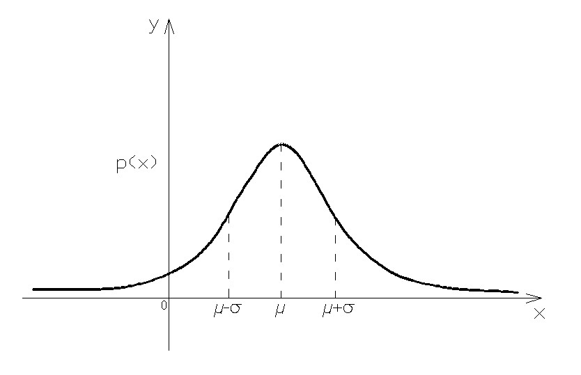
Normal distribution
The random variable Normal (also called random Gaussian variable or Gaussian curve) is a continuous random variable with two parameters, conventionally indicated with:
![]()
It is one of the most important random variables, especially continuous, as it is the starting base for the other random variables (Chi Square, Student t, F Snedecor etc.).
The Gaussian random variable is characterized by the following probability density function, which often refers to the term Gaussian curve or Gaussian:
where x is the size of which we must calculate the probability
![]()
and where μ and σ represent the average population and the standard deviation. The equation for the density function is constructed such that the area under the curve represents the probability. Therefore, the total area is equal to 1.
One of the most noticeable characteristics of the normal distribution is its shape and perfect symmetry. Notice that if you fold the picture of the normal distribution exactly in the middle, you have two equal halves, each a mirror image of the other. This also means that one half of the observations in the data fall on each side of the middle of the distribution.
The midpoint of the normal distribution is the point that has the maximum frequency. That is, it is the number or response category with the most observations for that variable. The midpoint of the normal distribution is also the point at which three measures fall: the mean, median, and mode. In a perfect normal distribution, these three measures are all the same number.
Resorting to standardization (statistics) of the random variable, ie the transformation such that:
![]()
where the resulting variable
![]()
also has normal distribution with parameters μ = 0 and σ = 1, the curve of gauss can be written as:
![]()
The characteristic value can be estimated by using the expression:
![]()
With a probability of 5% Z (from the table) is equal to -1.645, so the above expression can be rewritten as:
![]()
Dividing both sides by the mean μ the relationship becomes:
![]()
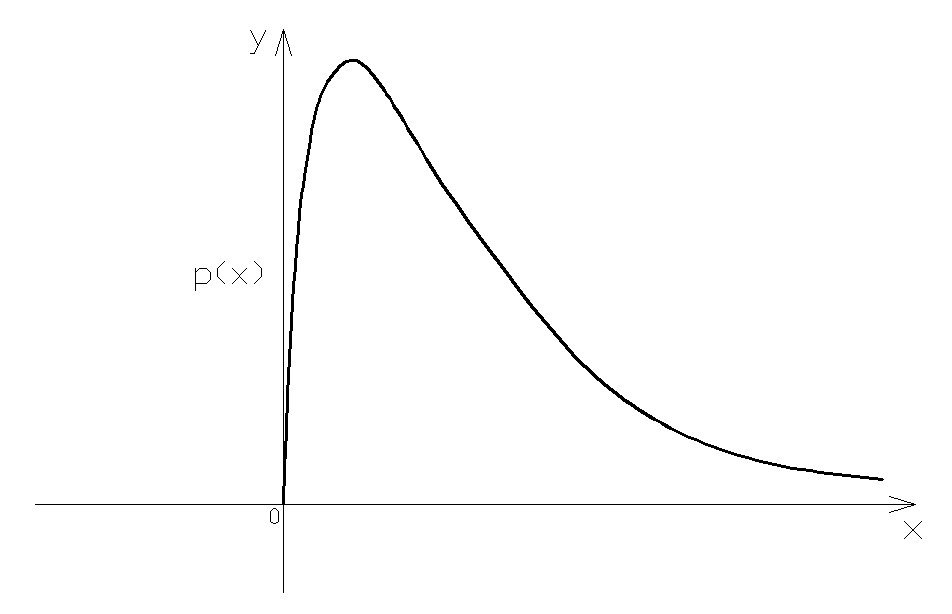
The lognormal distribution
A random variable x has a lognormal distribution with parameters μ eg, if ln(x) is normally distributed with mean μ and standard deviation s.
Equivalently:
![]()
and
![]()
where y is normally distributed with mean μ and standard deviation s.
The parameter μ can be any real, while s must be positive.
The distribution curve of the probability takes the following form:
Because of the asymmetry of the curve, the values of mean, mode and median do not coincide, unlike what happens instead in the normal distribution. The maximum point of the curve is, in fact, shifted to the left compared to the average value.
Student's t-distribution
The Student's t-distribution considers the relationship between the mean and variance in small samples, extracted from a normally distributed population, using the variance of the sample.
Given a normally distributed population, one draws a random sample of n observations, and calculate the random variable t, defined by the following equation:
![]()
where s is the sample variance.
t follows a Student t law with n-1 degrees of freedom. The quantity in the numerator is called the standard error of the sample.
The shape of the distribution depends on the degrees of freedom, ie, by the size of the sample. For large n (>30) t tends to a normal.

Rule of three-sigma
In a normal distribution 99.73% of the measurements fall at a distance from the mean value of three times the standard deviation, ie there is a probability of 99.73% that a measure drawn randomly from the population lies within ± 3s compared to the average m.
Once known the highest value measured in the population given by:
![]()
and the lowest:
![]()
the standard deviation of the population can be calculated as:
![]()
Bayes' Theorem
Bayes' theorem, proposed by Thomas Bayes, stems from two fundamental theorems of probability: the probability theorem and the absolute probability theorem. It is often used to calculate the posterior probabilities given by observations.
This theorem can be expressed as:
![]()
Where:
•P(A) the prior, is the initial degree of belief in A (the probability that event A occurs)
•P(A\B) he posterior, is the degree of belief having accounted for B (the probability that event A occurs if event B occurs)
•P(B\A) the probability that event B occurs if event A occurs
•P(B\A’) the probability that event B occurs if it doesn't occur the event A=1-P(B\A)
•P(A’) the probability that it doesn't occur the event A=1-P(A).
|
©GeoStru