Interfacing between the slices
With this method, the soil is modeled as a series of discrete elements, which we will call "slices", and takes into account the mutual compatibility between the slices. A slope in the present model is treated as comprised of slices that are connected by elastoplastic Winkler springs. One set of springs is in the normal direction to simulate the normal stiffness. The other set is in the shear direction to simulate the sliding resistance at the interface. The behavior of the normal and shear springs is elastoplastic. The normal springs do not yield in compression, but they yield in tension, with a small tensile capacity for cohesive soil (tension cutoff) and no tensile capacity for frictional soil.
The shear springs yield when the shear strength is reached. For brittle soil, the peak strength of the shear springs is determined by:
![]()
while the residual shear strength given by:
![]()
For simplicity, in the following analysis, it is assumed that after reaching the peak strength, the soil resistance drops immediately to the residual strength value.
For plastic non brittle soil, the strength does not reduce at large shear deformation; thus, the residual strength has the same value as the peak strength. The formulation of the present method follows that of previous research of Chang and Mistra on the mechanics of discrete particulates.
Let uia, uib, e ωa, ωb represent the translations and rotations of slice A and slice B, respectively. Let P be the midpoint of the interface between these slices. The displacement of slice B relative to slice A, at point P, is then expressed in the figure below, where riap the vector joining the centroid of the slice to location P. The displacement of the slice A in the point P is expressed as follows:
If slice B is immovable, the values of uxb, uyb, e ωb taken equal to zero .
Let nip be an inward vector normal to the side face of slice A at point P, defined as nip = (cosα, sinα ) where α the angle between the x-axis and the vector nip . The vector sip, perpendicular to the vector nip, will be defined by sip = (-sinα, cosα)
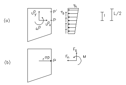
Figure 7.1.1 (a) shear and normal stresses; (b)Equivalent forces and moments between adjacent slices.
The displacement vector of the first member of the equation 3 can be transformed from X-Y coordinates in local coordinates n-s as follows:
Due to the relative movements of two neighboring slices , for a generic point P' of the interface, at a distance l from the central point P like in the figure 7.1.1, the the spring stretch in the normal direction dn and in the shear direction ds are given by:
![]()
As a result of spring stretch, normal and shear stresses on the slice interface are generated as shown in the figure 7.1.1. These stresses on the interface can be integrated to obtain the resultant forces and moment as follows:
where
kn = spring constant per unit length of the normal spring
ks = spring constant per unit length of the shear spring
L = length of the interface
Note that the springs are elastoplastic so the values of kn and ks are function of the deformation, so they must be obtained from stresses-deformations represented in the figure 7.1.2. For non-yield interfaces elastic spring constants kn and ks are used. For a yield interface, elastic constants are no longer applicable, and a method that considers the nonlinearity of the problem is required. In this regard, a secant stiffness method is employed. The equivalent spring constants ` kn and ` ks for a yield interface can be obtained that corresponds to the deformation of the interface like in the image 7.1.2.
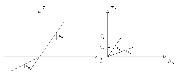
Figure 7.1.2 Secant stiffness method for obtaining 'Kn 'Ks
Integrating these expressions, since the terms that include the first order KnL are zero we obtain:
or, in matrix form:
where:
For convenience, the side forces FnP and FsP in the local coordinate system n-s are transformed to FxP and FyP in the global coordinate system X-Y as shown in the following:
The forces acting on all sides of a slice should satisfy the equilibrium requirement, given by:
where N is the total number of sides of the slide. The force fxa, fya is the weight of the slice acting through its centroid. The body force fxa and moment ma of the slice are usually equal to zero. Combining (3), (4), (9), (10) and (11) we obtain a relationship between the forces and the movements of the slice in the following form:
the matrix [c] is given by the multiplication of the following matrices:
Based on (12), three equations of force equilibrium can be set up for each slice, obtaining a system of 3 x N equations for N slices, expressed as follows:
![]()
{ f } : is composed by fx, fy and m, for each slice
{ u } : is composed by ux, uy ed ω, for each slice
[G]: the total stiffness matrix.
There are six variables for each slice, body forces fx, fy , moments m, movement ux, uy and rotation ω, in which two body forces and one moment are known: fx = 0, fy is the weight of the slice and ω = 0.
Therefore, the set of 3N simultaneous equations can be solved for the 3N unknown variables: ux, uy and ω of each slice.
Then the relative movement of two adjacent slices can be determined by (3), and the normal and shear forces between slices can be obtained from the force-displacement relationships (equations 4 and 9).
The normal stress σn and shear stress τs on the base of each slice can be determined by dividing the force by the area of the base:
© GeoStru