§ 7.4.3(1)P states that when a calculation is deemed necessary, the deformations shall be calculated under load conditions which are appropriate to the purpose of the check.
The calculation method adopted by the program is the most rigorous outlined in §7.4.3(7): curvatures are evaluated at frequent sections along the member and then are calculated the deflections twice, assuming the whole member to be in the uncracked and fully cracked condition in turn, and then interpolate using the following expression:
α = ζ αII + (1 - ζ) αI (7.18) EC2
where
α is the deformation parameter considered which may be, for example, a strain, a curvature, or a rotation
αI, αII are the values of the parameter calculated for the uncracked and fully cracked conditions respectively
ζ is a distribution coefficient (allowing for tension stiffening at a section) given by the expression:
ζ = 1 - β (σsr/σs)2 (7.19) EC2
β is a coefficient taking account of the influence of the duration of the loading or of repeated loading
= 1.0 for a single short-term loading. Program assumes this value when Characteristic or Frequent comb. option is checked
= 0.5 for sustained loads or many cycles of repeated loading. Assumed by program when Quasi-permanent comb. option is checked
σs is the stress in the tension reinforcement calculated on cracked section
σsr is the stress in the tension reinforcement calculated on a cracked section under loading causing first cracking
σsr/σs = Mcr/M = fctm/σct,min where Mcr is the cracking moment; σct,min is the min concrete tension in the uncracked section
For loads with a duration causing creep, the total deformation including creep may be calculated by using an effective modulus of elasticity for concrete according to:
Ec,eff = Ecm / (1+φ(∝,t0)) (7.20) EC2
where
φ(∝,t0) is the creep coefficient relevant for the load and time interval
If in the input window you select the option "Characteristic comb." only short-time deflection are calculated. If, instead, you select "Quasi-permanent comb." long-time deflection are calculated using the age adjusted effective modulus (see AAEM method):
Ec,eff(∝,t0) = Ecm / (1+ c.φ(∝,t0))
where
c = aging coefficient: c(∝,t0): for t0 > 15 days that value may be assumed equal to 0.8 or 1.0 if you want to adopt the EM method suggested by (7.20) EC2.
The values of φ(∝,t0) and c must be assigned (changing the default values) in the Materials library of the sections of sub-element (one or more) that compose the beam. The same for the eventual shrinkage coefficient εcs (∝,t0) to take in account. Program do not use the relation (7.21) in EC2 but the unified theory outlined in AAEM method paragraph.
Serviceability limit value of deflection for beam, slab or cantilever subjected to quasi-permanent loads must not exceed span/250. For the deflections after construction, span/500 is normally an appropriate limit for quasi-permanent loads: in the case of partitions may be appropriate to calculate deflections (to limit at max span/500) as difference between total long-time (t=∝) deflection and the deflection due to self weight + dead load before partition construction (so we have to do two separate calculations).
Load history influences the value of deflections. A typical load history for building could be:
•Application of self weight g1 at time t1 (about 10 days)
•Application of remaining dead loads g2 (including partitions) at time t2 (about 60 days)
•Application of quasi permanent live load ψ02 ⋅ g3 at time t3 (365 or typically ∝)
A simplified method to avoid to use (because the load history) different values for coefficient φ is the simplified method in /8/; this method consists in the following definition of an equivalent creep coefficient φeq :
φeq= [g1 φ(∝,t1) + g2 φ(∝,t2) + g3 φ(∝,t3)] / (g1+g2+ψ02⋅g3)
∝ may be any time values in days.
Program do not compare the calculated deflections with their limit values assessed by the user.
Section deformations
Each sub-elements of the beam is divided in segments by means of an assigned (in the input window) length of discretization. The deformation of the section calculated in the middle of each segment is assumed constant for the whole segment. Program calculates two deformations value for each mean section:
1) Instantaneous deformation (short-time effects)
The state I is the uncracked state with unlimited tension strength of concrete with a1,b1,c1 as deformation parameters. We have a state II when under N,Mx force the section cracks assigning 0 value to tension strength of the concrete with a2,b2,c2 as deformation parameters. For eq. (7.18) EC2 the mean deformation of the section at time t0 is:
where
ζ = 1- β (fctm/fct,min)2
ζ = 0 if fct,min< fctm the section is not cracked under N, Mx forces
σct,min is the min concrete tension in state I under N,Mx forces in the uncracked section.
1) Long time deformation
Program calculate the increase of deformations Δa1, Δb1, Δc1 at state I due to creep and shrinkage by means of AAEM procedure. So the deformation at time t is:
cy 3 = a3 = a1 + Δa1
cx 3 = b3 = b1 + Δb1
εO 3 = c3 = c1 + Δc1
At state II Δa2, Δb2, Δc2 are the increase of deformation. Total deformations at time t are then:
cy 4 = a4 = a2 + Δa2
cx 4 = b4 = b2 + Δb2 (1)
εO 4 = c4 = c2 + Δc2
By means the distribution coefficient ζ we obtain the mean deformations at time t:
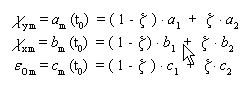
cy m = am (t) = ( 1 - ζ ) a3 + z a4
cx m = bm (t) = ( 1 - ζ ) b3 + z b4 (2)
εO m = cm (t) = ( 1 - ζ ) c3 + z c4
Deflections in single beam
Beam can be assigned as consisting as one or more sub-elements: each sub-element is characterized by a constant section (as geometry and reinforcement) and a distributed load acting on it. Two sub-element may be different only for different placing of longitudinal bars or for different distributed load. Before of this input it is necessary to input ad save with different names the above sections that define the different sub-elements (even a single). At each sub-element correspond a section that may be predefined or general but always with uniaxial bending forces. Pertinent creep, shrinkage and aging coefficients must be assigned to each section in Materials library and they are taken in account in the deflection calculation of the beam.
The beam can be hyperstatic as belonging to a frame, but solving the frame, for the combination of interest (usually quasi-permanent), we can make the beam isostatic (on two supports) applying the two hyperstatic bending moments at the end. This is a simplification that disregards the true interaction in the time of hyperstatic forces with creep and shrinkage effects: specific studies have shown that the difference in deflection is negligible.
Beam on two supports
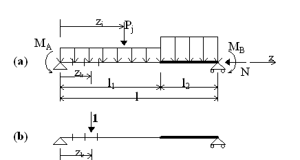
To fix the ideas with an example we show the calculation scheme in the above figure (a) that refers to a beam consisting of two sub-elements whose lengths are indicated as l1 and l2. The two sub-element have different sections and acting loads (self-weight shall be included in the distributed load). Bending moments MA and MB at the end of the beam may represent hyperstatic action from adjacent structural elements. Concentrated loads Pj may be assigned in any point of the span. A constant axial force N may be present (so we can also study, for example, the shortening of columns under creep effects in height buildings).
In uniaxial bending we denote with χ(z) the distribution of curvatures along the beam due to the acting loads in the scheme (a) and with M'(z) the bending moment produced by a unit load in the service scheme in (b) figure. The principle of virtual work gives the following deflection formulation for η at the abscissa z of application of unit load:
![]()
To resolving the integral in numeric form we subdivide the whole length of the beam in N little segments. Each segment has a length Δzk and abscissa of its mean point equal to zk. The numerical integration can be express:
![]()
If we substitute in the summation short-time values of curvatures χ of the sections we obtain the instantaneous (t=t0) beam deflections. Long-time deflection (t=∝)are obtained with the substitution of long-time values of curvatures.
Cantilever beam
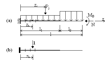
The same type of scheme and relationships has been applied to the cantilever typology of beam (very sensitive to bending deflections).