Given a cross-section referred to O,x,y axes, the bending is defined uniaxial when the bending is around x axis and the corresponding neutral axis is parallel to x.
This condition, strictly speaking, is true only if the section is symmetrical with respect to y axis. But in many circumstances (beam within rigid floor diaphragms, foundation beams) the lateral constrains make sufficiently approximate the above hypothesis.
To evaluate internal forces Mx, N for each position of the neutral axis program works with the following procedure of integration of stresses.
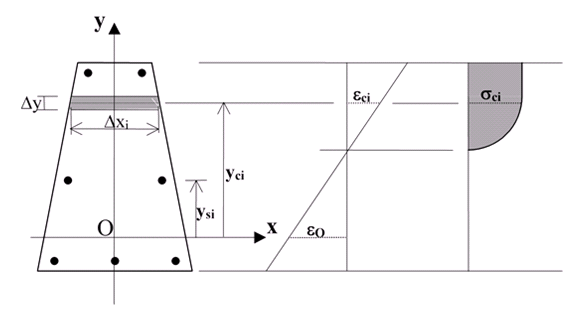
Discretization of cross-section and generic stain and stress distribution
The cross section is first discretizzed into n strips parallel to x axis (and then to neutral axis) having all the same thickness Δy (step) that you can change (from 0.2 to 2.0 cm) in the dialog window Code and reinforcement options. The width of Δxi each strip is given (see figure above) by the intersection of the line passing in the middle of the step Δy. The area of each strip is then given by:
Ac i = Δxi . Δy
The internal forces N , Mx for any position of the straight line of deformation of the cross-section are given by the following equilibrium equations referred to x axis:
where:
σci is the stress, assumed constant in the entire strip, in the Aci area
εci is the strain, assumed constant, in the Aci area
σsi is the stress in the centroid of area Asi of the generic bar i
εsi is the strain in the centroid of area Asi of the generic bar i
In above summations the normal force N is supposed to be applied in the origin O; to compare the internal moment Mx with the external one (design moment) with N placed in the centroid of concrete section, it is necessary (after summation) to add the moment - N yC to the above Mx (YC = y-coordinate of centroid).
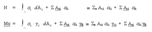
Every possible strain distribution in ultimate limit state is shown in the figure below.
All possible strain distribution at ultimate limit state (with strength areas between 1-2-3-4 characteristic points)
For the assumption of conservation of planar sections and the described limitations imposed to the ultimate strain of concrete and steel, the deformed configurations of the section, corresponding to the various possible ultimate states, all pass at least one of the points labeled A, B, C of the figure. In the same figure are also represented the positions 1-2-3-4 (for positive curvatures) of the strain configurations corresponding to transition from one type of failure to another.
The strength area from 1 to 2 is obtained by rotating the section around the point A (pivot A). The second area from 2 to 3, by rotating the section around B. The third field, finally, from 3 to 4 around the pivot C.
SAFETY CHECK
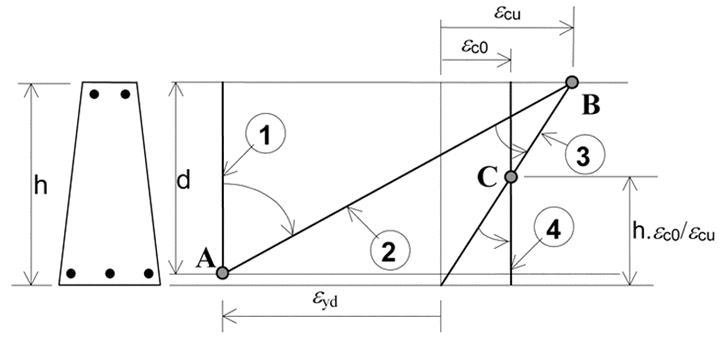
Strength domain (interaction N-Mx domain) for ultimate limit state in uniaxial bending
The above figure is a generic interaction region of the strength internal forces N, Mx (the moment is referred to the centroid of concrete).
The boundary curve of region is the border of strength domain and each of its points corresponds to one of strain distribution (with εc or εs at their strength value) shown in previous paragraph.
In that border 1-2-3-4 points are the same points seen in the previous topic with only reference to the positive (2-3) or null (1-4)curvatures. Points 5-6 refers to negative curvatures.
To calculate the forces N, Mx corresponding to those characteristic points (from 1 to 6) just executes the integration described in the topic uniaxial bending assuming the following analytical expression of the straight line of deformation:
ε(y) = b y + c (1)
where :
b = cx = curvature around x axis
c = eO = strain in the origin O of reference axes x,y
coefficients b, c of line (1), are derivate by the strains εP , εQ of any two points P,Q of the section with y-coordinates yP, yQ:
b = (εP - εQ) / ( yP - yQ)
c = εQ - b yQ
Known b, c it is easy to calculate with the eq. (1) any point {N,Mx} of the safety border. For example if you want an intermediate point between characteristic points 2 and 3 of which are known the curvatures b2, b3 referred to pivot B (in previous topic):
assign a generic curvature b between b2 and b3, indicate with yB, εB the y-coordinate and the known strain of pivot B, you can get the unknown value of coeff. c in eq. (1):
c = εB - b yB [ b2 < b < b3 ]
The integration of stress provides, finally, the pair of N, Mx values of point with curvature b.
c = εB - b yB [ b2 < b < b3 ]
The same procedure you can do for every b curvature for the other characteristic couple of points so to built the entire border of the strength domain.
Given a generic couple of design forces {NS,MxS}, uniaxial bending check is positive if its representative point S (see previous figure) is not external to strength domain (as in depicted case). This condition that we define measure of safety can be numerically expressed in multiple ways. This program allows the following two way (see previous figure):
1) At constant eccentricity e=Mx/N: program calculate {NR,MxR} of point R as intersection of border line with the stress path line r (with Mx/N = e for all of them). The measure of safety is given by the segment ratio OR/OS (Safety Factor). If such ratio is ≥ 1.0 the bending conformity is positive for {NS,MxS} design forces.
2) At constant normal force N=const.: program calculate {NR',MxR'} of point R' as intersection of border line with the stress path line r' (with N = const for all of them). The measure of safety is given by the segment ratio O'R'/O'S (Safety Factor). If such ratio is ≥ 1.0 the bending conformity is positive (check is OK) for {NS,MxS} design acting forces.
DIRECT SAFETY CHECK
Program perform the uniaxial bending check (to obtain the safety factor) in the following way.
Generic equation of straight line r (or r') in the previous figure has the form:
l · N + m · Mx + p = 0 (2)
where l, m coefficients are immediately given from condition that r passes through the design point {NS,MxS} and the origin point O (or O')
In the case depicted in the previous figure the intersection point {NR,MxR} R is placed between characteristic point 2-3 then in the second area strength then we know the pivot B:
the only unknown is then the curvature b that must be: b2 ≤ b ≤ b3. So b can be easily calculated with iterative procedure of bisection.
|
© 2020 Geostru