Granulometry allows the input of data from particle size analyses conducted in the laboratory. For coarse-grained soils, sieving data can be loaded, while sedimentation analysis is available for fine-grained soils.
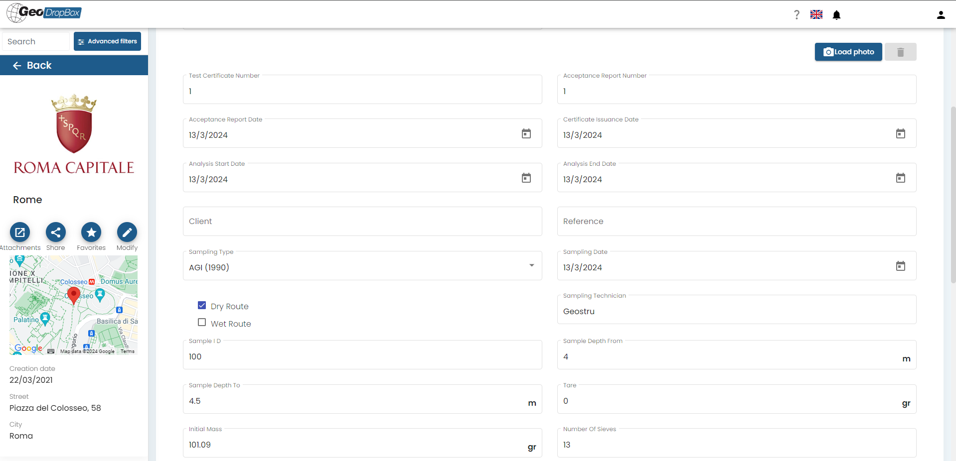
This test enables the input of various descriptive data including:
•Test certificate number
•Acceptance report number
•Date of acceptance report
•Certificate issue date
•Analysis start date
•End date of analysis
•Client
•Reference
•Sampling Type: establishing criteria or standards for soil type subdivision based on grain diameter
•Sample opening date
•Dry/Wet route: indicating whether the sample was analyzed via a dry or wet route
•Name of Sampling Technician
•Sample Id: unique sample number
•Sample Depth: starting and ending depth (in meters) from which the sample was taken
•Tare weight (if applicable) in grams
•Initial mass (grams)
•Number of sieves used for the analysis
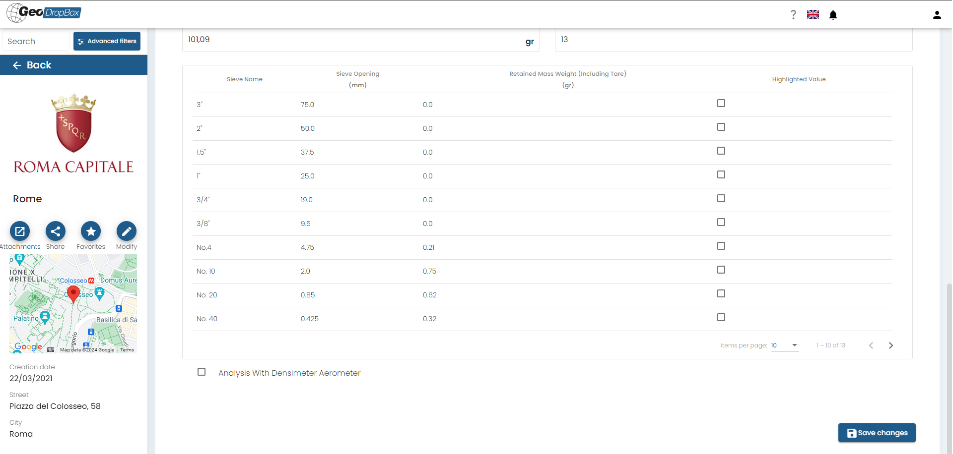
Once the mandatory data is entered, GeoDropBox generates rows corresponding to the number of sieves used. Each row includes four columns for input:
•Sieve name (optional)
•Sieve opening (mm) (mandatory)
•Weight Retained mass (including tare) (grams) (mandatory)
•Highlighted value: if selected, displays the screen highlighted in the report.
Finally, the following are calculated:
•Uniformity coefficient U given by the relation D60/D10
•Curvature coefficient C given by the relation D302/(D10*D60)
•Permeability coefficient K (cm/sec) (valid for uniform sands - Allen Hazen) given by the relationship: C* D102 (where C is the Hazen constant set equal to 100 if the permeability expressed in cm/sec, 0.01 if expressed in m/sec)is if D10<=2 otherwise "--"
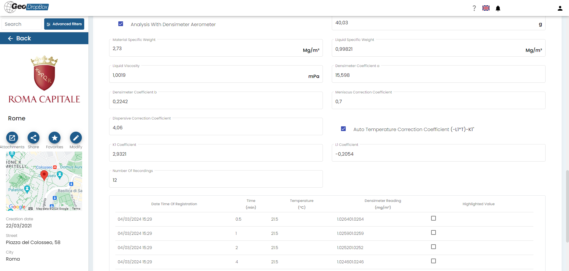
By ticking the option "Analysis with Densimeter", it is possible to enter data for the analysis for fine-grained soils, if the weight of the soil passing through the last sieve is a significant amount.
For this analysis, the equivalent grain diameter is calculated with the relation:
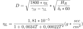
Where:
HR = Densimeter Report will be given by:
HR = a - b*Rh
in which in turn:
•a and b are coefficients given by the densimeter report;
•Rh is the densimeter reading corrected by the meniscus coefficient;
•η is the viscosity of the liquid expressed in Mpa;
•γs is the specific weight of the material expressed in Mg/m3;
•t is the time interval expressed in minutes.
In the calculation of D the term HR appears as seen, the value of Rh would be the corrected densimeter reading set equal to (r-1)*1000 (where r is the density reading read on the instrument) to which is added a coefficient Cm (meniscus correction) which is usually set equal to 0.5
So you will have:
R’=Rh=(r-1)*1000+Cm (2)
Meniscus correction (Cm): The densimeter is calibrated to measure the density of the suspension at level A. The densimetric reading is taken at the top of the meniscus (level B). The difference in values between levels B and A is referred to as the meniscus correction (Cm). Typically, Cm values hover around 0.5 (AGI, 1994). Cm is always added to the Rh value. The resulting R' value, obtained by adding Rh and Cm, represents the 'true densimetric reading'.
Temperature correction (Ct): Generally, densimetric measurements should be conducted at a temperature of 20°C. If the test is conducted at a different temperature, the density of the water and the density measured by the densimeter in the solution may vary. These discrepancies are rectified using a correction factor Ct. Ct is added to R'.
Ct= -K1-L1*T (3)
where K1 and L1 are the coefficients derived from the linear regression line entered by the user.
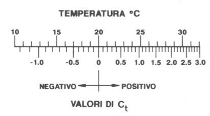
During the reprocessing of the data provided by the densimeter, it was found that, at times, even when using the correction coefficient for temperature, the percentages of material retained in an ideal sieve with a diameter corresponding to that evaluated with the Stokes formulae, could be greater than 100 %, even if for values of less than 1% . To overcome this absurdity, in such cases it became necessary to use a second temperature correction method, provided by Head (1970), which involves the use of an abacus, as illustrated in figure
Dispersant solution correction (Cd): The presence of the antiflocculant inside the test solution causes an increase in the density of the liquid, thus affecting the densimetric reading. To determine the correction coefficient Cd, a 5*104 mm3 volume of the compound is placed inside a calibrated container; this volume is dried at 105-110 °C and the mass md (in grams) of the dispersing agent is measured.
The correct reading is then obtained as:
R’’= R+Cm+Ct-Cd (4)
R’’=(r-1)*1000+Cm+Ct-Cd (5)
Once the densimeter reading has been corrected and the grain diameter has been obtained, the percentage of retained and passing grains can be calculated as:
% retained = R’’*(100/Pps)*[γs/(γs-γ)]
% passer = % retained*% of material remaining from the coarse grain test
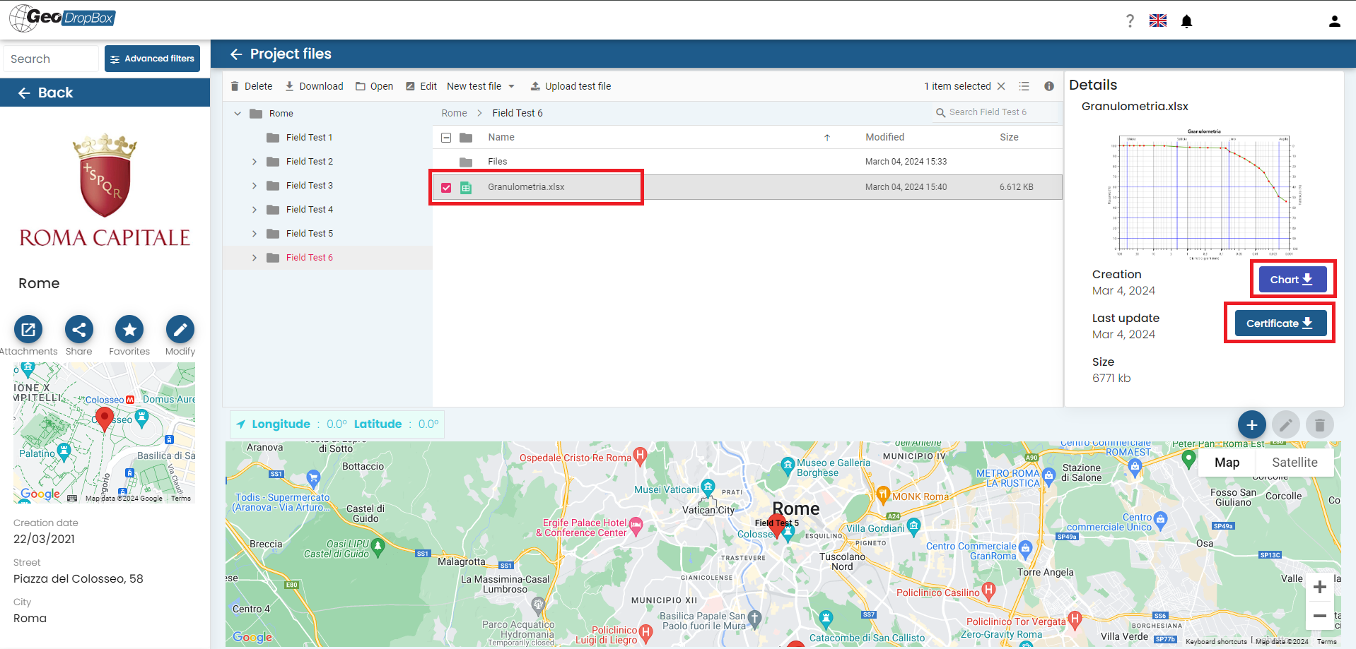
After clicking "Save Changes," the particle size curve and the file "Granulometry.xlsx" containing all the entered data will be generated. By selecting the file and clicking "Open," the comprehensive analysis report will be displayed.
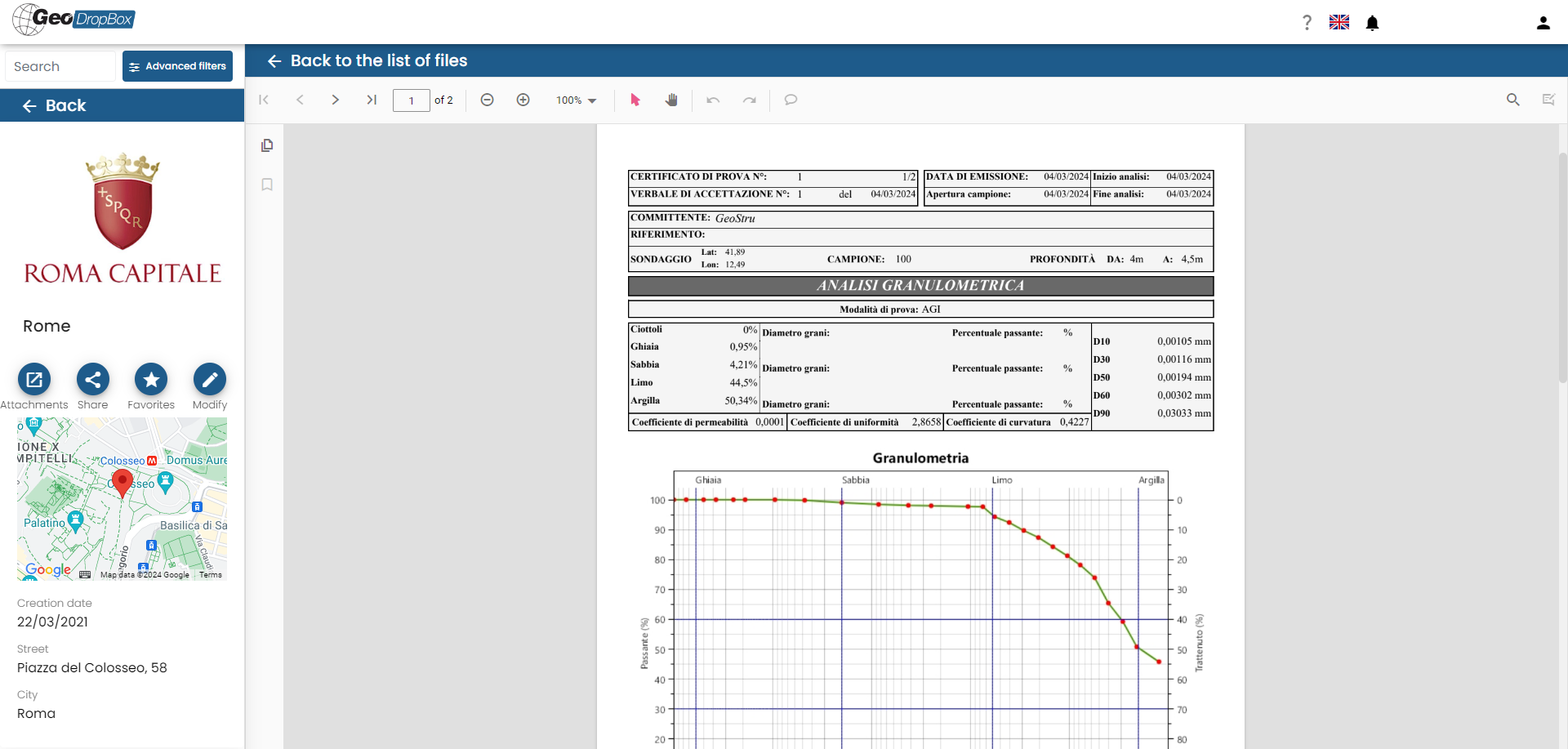
You can also download the image file of the particle size curve by pressing "Chart" and the test certificate in *.pdf format by pressing "Certificate":
© GeoStru