After computing the element matrices and vectors, the assembly process is used to compute the global equation system. Solution of the global equation system provides displacements at nodes of the finite element model. Post processing of the results is then required to calculate the strains and stresses in each element. For elasticity problems, the strains in an element are calculated from the displacements by:
|
|
(52) |
In simplex elements (CST-T3 for instance) the strain-displacement matrix B is a constant, and the strains are constant, and therefore can be computed anywhere in the element. For the higher-order elements, however, B is a function of the coordinate system (displacements) and not always explicit. Therefore the strains must be evaluated at specific positions in such elements. The most accurate locations are the sampling points used to calculate the strain-displacement matrix B and the stiffness matrix k.
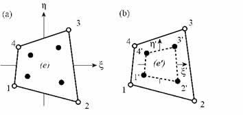
Stresses are calculated with the Hook's law. These stresses can be computed anywhere in the element but have best precision at the Gaussian integration points used for the stiffness element formulation. For instance for the 4-noded quadrilateral element the stresses have best precision at 2x2 integration points as shown in the Figure 23.
|
Fig.23. Extrapolation from 4-node quadrilateral sampling points; (a) 2 x 2 rule. (b) Gauss element (e') |
In order to build a continuos field of stresses it is necessary to extrapolate result values from the integration points to the nodes of the finite element. The stresses of the nodes, particularly those at the corners of the element, are more useful. To calculate the nodal stresses, either the B matrix must be calculated at the nodes, or the stresses must be interpolated from the values at the sampling points. A possible way to create continuos stress field with reasonable accuracy consists of: 1) extrapolation of stresses from reduced integration points to nodes; 2) averaging contributions from finite elements at all nodes of the finite element model. The interpolation-extrapolation process is described as follows.
Let’s assume that stresses have been computed at the four Gauss points of a 4-noded quadrilateral plane element (points 1’, 2’, 3’ and 4’). We now wish to interpolate or extrapolate theses stresses to other points in element. In Figure 23 the coordinate ξ’ is proportional with ξ and η’ with η. At point 3’ ξ’=1 and η’=1 and ξ=η=1/√3. That is
|
|
(52) |

Stresses at any point P in the element are found by the usual shape functions assumed for the displacement field interpolation:
|
|
(53) |
where σ is σx, σy, τxy respectively. The shape functions Ni are the bilinear shape functions:
|
|
(54) |
The shape functions are evaluated at the ξ’, η’ coordinates of point P. For example, let point P coincide with corner A. To calculate stress σx at this node from σx calculated at the four Gauss points we substitute ξ’= η’=√3 into the shape functions defined above and apply the formula given by the Eq.(53).
In the cases of triangular elements similar approach is applied. For instance for higher order 6-noded triangular finite element and three sampled Gauss points the stresses at any point in the element are computed using the shape functions as:
|
|
(55) |
where the shape functions Ni
|
|
(56) |

are computed at the ξ’, η’ coordinates:
|
|
(57) |

As already stated these quadratures are lower order for higher order elements and repsesents the so called reduce integration scheme. The reduced integration scheme may be desirable for two reasons. First since the expense of generating a finite element matrix by numerical integration is proportional to the number of sampling points, using fewer sampling points means lower cost. Second, a lower-order rule tends to soften an element, thus countering the overly stiff behavior associated with an assumed displacement field. Stresses are usually averaged at nodes in FEA software to provide more accurate stress values. This option should be turned off at nodes between two materials or other discontinuity locations where discontinuity does exist. The stresses and strains at the centre of the element will be obtained through extrapolation of the stresses from the Gauss integration points.
|
Fig. 24. Super convergent Patch Stress Recovery. |
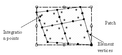
Moreover in the computer program is implemented a very efficient technique called Super Convergent Patch Stress Recovery (SCP). Basically the method use the concept of the local patch of elements sampled at their integration points to yield a smooth set of least square fit nodal stresses (Fig. 24). As noted earlier, the integration points are special points where the stresses have the best values, those gradient locations match those of polynomials of one ore more degrees higher.
|
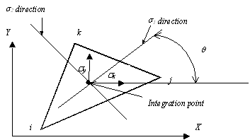
Fig. 25. Principal stresses. |
The user is often interested not only in the individual stress components, but in some overall stress value such as Von-Misses stress. In case of plane stress, the Von-Misses stress is given by:
|
|
(58) |
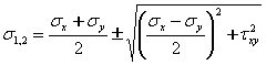
where σ1 and σ2 are principal stresses given by:
|
|
(59) |
The angle formed by the principal stresses directions may be also computed (Fig. 25):
![]()
The postprocessor display the stress contour, which typically are smoothed by working from nodal average stresses. These contours may be plotted as “stress bands” by designating equally spaced stress intervals, locating the areas of each element that fall into each interval, and using different colour to plot each interval.
|
© GeoStru Software