<< Click to Display Table of Contents >> Navigation:  Nonlinear analysis formulation > Elastic-plastic procedures > Tangent (variable)-stiffness method

 

The second approach, shown in Figure 43, takes account of the reduction in stiffness of the material as failure is approached. If small enough load steps are taken, the method can become equivalent to a simple Euler "explicit" method. In this approach the global stiffness matrix may be updated periodically and "residual body-loads" iterations employed to achieve convergence. In contrasting with "constant stiffness approach" the extra cost of reforming and re-factorization the global stiffness matrix in the variable stiffness method is offset by reduced numbers of iteration, especially as failure is approached.

The algorithm requires that representation of the stress-strain relation must be stored, so that tensions and elastic constants can be obtained for any given deformation. We also have to store and update at any sampling point of each element after each computational cycle, element strains and stresses and the nodal displacements.

An incremental relationship between displacement and force is needed:

 

                                                 

where Kt is the tangent stiffness matrix and the above equations represent the linearized eqauation of the nonlinear equation 191:

 

             

 

 

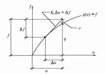
The computation proceeds by applying a load increment ΔF and computing the corresponding displacement increment from equation (190) (Fig.43).

The strain increment is computed in the usual way as:

 

                                                     

Next the stresses are computed via the elasto-plastic constitutive relation:

 

                                                                                       

This is a nonlinear relation since the constitutive matrix Eep depends on the current stress state and generally iterative procedures must thus be used. Assuming that the stresses have been computed the internal force vector can then be found as:

 

                                                           

this must be balanced by the total applied load, therefore the residual force must vanish:

 

                                                   

If the residual is different from a given tolerance it is applied as an external load following the well-known Newton-Raphson procedure. This then gives a new strain increment and a corresponding new stress increment, which must be determined via the nonlinear elasto-plastic constitutive relation, a new residual is computed and so on until the residual becomes sufficiently small. The procedure can be outlined as follows:

 

1.     Apply load increment ΔF and find displacement and strain increments Δu and Δε

2.     Determine stress increment Δσ from equation (193)

3.     Compute residual R.

4.     If set and goto 1

 

Thus, the computation of a load step requires a global iterative procedure where the out of balance force, or residual, must vanish, as well as a procedure to compute the stress increments (step 2). The stress update is performed in each integration points. In order to compute the stress increment given a strain increment the backward integration scheme is implemented in the code. Essentially the method consists of an elastic predictor, followed by a plastic corrector to ensure the final stress is nearly on the yield surface.

 

 

 

 

 

 

 

 

 

© 2020 GeoStru Software