<< Click to Display Table of Contents >> Navigation:  Introduzione > Terrain 4 SDK

Specifiche tecniche di elaborazione

---

Principi di un DTM

Triangolazione di Delaunay

Triangolazioni vincolate

Voronoi Diagrams

Gridding

Anisotropic Meshing

Kriging

Custom variograms

References/bibliography

 

Principi di un DTM

---

Un modello digitale del terreno è per definizione un  insieme di dati che permette l'interpolazione di un punto arbitrario di terreno con una precisione prefissata. In tal senso il DTM si distingue sostanzialmente dalle linee di contorno o curve di livello di una mappacarta. Le curve di livello e i contorni forniscono unicamente un'informazione di elevazione di altezza sull'elemento linea stesso: inoltre, l'immagine delle linee di livello dovrebbe consentire un'impressione della morfologia del terreno (terreno liscio poco ondulato, linee lisce smussate, terreno scabro, linee fortemente ondulate, ecc.). Le linee curve di livello dovrebbero inoltre rappresentare lievi e piccole caratteristiche geomorfologiche attraverso la loro forma tipica e "l'effetto famiglia". Ciò a volte richiede un'esagerazione di certe forme del terreno. Di conseguenza, le linee di livello sono intese specialmente per la visualizzazione del terreno, mentre i dati per un DTM sono destinati a fornire informazione circa l'elevazione e l'andamento delle quote dell'intero in ogni punto del terreno in una forma leggibile dal computer. Le curve di livello ottenute da un dataset di un DTM non mostreranno in modo specifico la morfologia del terreno analogamente a quelle dei profili disegnati da un topografo.

 

Dati di base per un DTM e principi di interpolazione. Triangolazione di Delaunay

---

I dati necessari per un DTM sono punti sparsi (mass points) e linee caratteristiche come break lines, linee di strutturali del terreno, talweg, delimitazione contorni di zone morte non cartografabili (dead areas) e altri. In generale, per interpolazione la quota di un punto viene calcolata attraverso l'interpolazione lineare fra punti contigui. Una tecnica molto comune consiste nell'eseguire una triangolazione fra i punti di appoggio rilevati. Ciò significa che si definisce una serie di triangoli in cui i punti angolari dei vertici sono i punti sparsi. Molto spesso viene utilizzata la triangolazione di Delaunay; in questo caso si sceglie il cerchio più piccolo contenente solo 3 punti contigui. All'interno di questo triangolo si interpola utilizzando generalmente tecniche bilaterali bilineari, ma occasionalmente si utilizzano anche tecniche bi-cubiche. La triangolazione non può passare sopra o attraversare una linea caratteristica. Le linee poligonali spezzate delle linee caratteristiche vengono sempre utilizzate come linee del triangolo fatte coincidere con i lati dei triangoli .

 

Triangolazioni vincolate

---

I punti sparsi o un reticolo sono destinati a rappresentare il terreno naturale ma riprodurranno caratteristiche di terreno diverse quali bordi e discontinuità del terreno, ubicazione di dighe, solo in modo alquanto incompleto. Si raccomanda quindi di utilizzare break lines o linee di vincolo  per tutte le varie caratteristiche di terreno che eccedono la precisione di quota del DTM entro punti di griglia contigui di una maglia del grigliato.

Dovranno essere indicate in modo speciale le zone di minor precisione in quanto coperte da vegetazione o da altri ostacoli, nonché le zone che non possono essere misurate. Nei DTM con precisione inferiore al metro, sarebbe opportuno delimitare anche le zone che non dovrebbero essere segnate sulla mappa incluse nel DTM, perchè non appartenenti al terreno (case, laghi..).

Sono chiamate Triangolazioni vincolate tutte le triangolazioni che prevedono elementi strutturali sui quali i triangoli che si andranno a formare seguiranno un criterio imposto dal vincolo stesso.

 

Delaunay Triangulation

---

We define a triangulation of a finite set of points V in the Euclidean plane to be a maximal planar straight line graph having V as the set of vertices and such that no two edges of the graph properly intersect (i.e. only at their endpoints).

Terrain 5 model terrain using either a regular grid structure or a Triangle Irregular Network (TIN). The advantages of using a TIN are: triangles are simple geometric objects which can be easily manipulated and rendered; TINs are not bound by the regularity constraints of a regular grid and so can approximate any surface at any desired tolerance with a minimal number of polygons; multiple TINs of a single area of terrain can be organised into a hierarchy with respect to their resolution so that they can provide generalizations or details as required by different applications. Of prime importance is that the triangulation is a good approximation to the real-world surface. A second requirement of the triangulation algorithm is that it should produce triangles which are as close to being equiangular as possible. This condition is essential for numerical interpolation since it ensures that the maximum distance from any interior point to a vertex of its enclosing triangle is reduced and it also minimises the aliasing which can arise when long, thin triangles are displayed. Thirdly, we need an algorithm which will produce a unique triangulation of a given set of points so that we generate reproducible and consistent surfaces. A Delaunay Triangulation provides all of the these benefits.

TINs main drawback is that no overhanging features can be represented, but this is usually a minimal concern with terrain. For representing overhanging features, a full blown 3D triangulation must be used.

Terrain 5 uses Delaunay triangulation for immediate use, or as a basis for for mesh smoothing, refining or resampling. Other kinds of mesh can be derived too, like grid meshes or bezier surfaces.

 

Voronoi Diagrams

---

Informalmente, un diagramma di Voronoi (anche conosciuto come Dirichlet o Theissen tesselation), rappresenta le regioni di un piano che sono vicine ad un particolare punto piuttosto che ad altri. Il diagramma di Voronoi ha maggiore importanza in problemi di geometria computazionale, ad esempio, può essere usato per risolvere problemi nearest neighbour di cui è dato un numero di punti.

Per cancellari i dati di voronoi prodotti dal programma accedere alla finestra "Gestore DTM", e nel pannello "Elementi del DTM" premere il pulsante "cestino" a fianco della vce "Voronoi".

 

Delaunay triangulation and Voronoi tesselation of space

---

Voronoi Diagrams are closely related to Delaunay Triangulations.

Delaunay (1934) proved that when the dual graph of a Voronoi diagram is drawn with straight lines, it produces a planar triangulation of the Voronoi points P (if no four sites are cocircular). This arrangement is called the Delaunay triangulation of the points.

A Delaunay triangulation is desirable for approximation applications because of its general property that most of its triangles are nearly equiangular and also because it generates a unique triangulation for a given set of points.

The properties of a Voronoi Diagram V(P), of a set of points P={P1,P2,...,Pn}, and its relationship to its corresponding Delaunay Triangulation, are as follows (after O'Rourke 1994):

•each Voronoi region V is convex

•if v is a Voronoi vertex at the junction of regions R(P1), R(P2) and R(P3) then v is the centre of the circle C(v) determined by P1 , P2 and P3

•C(v) is the circumcircle for the Delaunay triangle corresponding to v

•the interior of a circumcircle C(v) contains no points

•if Pj is a nearest neighbour to Pi , then P(i,j) is an edge of V(P)

•there is some circle through Pi and Pj which contains no other points, then (Pi,Pj) is an edge of V(P)

 

Grids

---

A grid G is a regurlaly spaced distribution of points Pg() in the Euclidian plane, each point being affected with a height data. A simple mesh can be derived from it as a maximal 3D straight line graph having with Pg() as vertices. Each point Pg() isn't coincident with any original point of P(), but is resulting of a local interpolation of P().

The process of estimating values at evenly spaced grid nodes based on the original irregularly spaced data is called " interpolation". There is no perfect solution to estimate values at each grid node and many techniques are in use. The validity of each depends on the type of data being interpolated and its distribution pattern. Triangulation is most commonly applied to elevation data since it is a technique that uses the slope between data points to estimate new grid values.

Grids are simple structures that can be easyly manipulated, they are, in essence, much like rasters. Unlike TINs, grids are bound by the regularity constraints and so can't approximate any surface at any desired tolerance.

Grid main drawback is it's inhability to represent overhanging features, or any feature topologically shorter than the cell size of the grid. Minimizing the cell size improves terrain representation, but induce an important growth in cells count, hence maximizing rendering time and storage space.

 

Anisotropic meshing

---

As in Ruppert's algorithm, the program eliminates "encroached" segments by inserting vertices at their midpoint. The only difference is that encroachment is verified after applying the transformation T assigned to the midpoint of the segment.

Then, the program locks every segment, determines what is the interior region, and starts attacking internal triangles of low quality by refinement (i.e. by inserting new vertices).

When grading is used, the quality of a triangle is defined to be its minimum distorted angle. When grading is not used, large triangles are penalized by dividing the minimum angle by the (distorted) perimeter of the triangle, squared. The power at which the perimeter is raised controls how much importance is given to the size of the triangle versus its shape. The current value was arbitrarily chosen to give pleasing results.

In Ruppert's algorithm, low quality triangles are removed by inserting a vertex at the circumcenter of the triangle. In the isotropic case, the triangle is Delaunay, therefore its circumcircle is empty and the circumcenter is a good place to insert a vertex. Furthermore, a Lemma guarantees that the circumcenter falls in the inside region (using the fact that the input is segment-bounded and that no segment is encroached). However in the anisotropic case there are some problems: the circumcircle is not necessarily empty. The circumcenter may fall arbitrarily close to another vertex or edge, or may even fall in the outside region. The program solves these problems by checking if the nearest neighbor of the circumcenter is a vertex of the triangle in question (as it would be in the isotropic case). If this does not hold, then we walk toward the centroid of the triangle and try again. After some number of consecutive failures, the program finally uses the centroid.

 

Kriging

---

Si tratta di una tecnica statisticamente complessa, stocastica, di tipo esatto, e si basa sulla teoria delle variabili regionalizzate di Krige. Richiede l'analisi preliminare del fenomeno per verificare se le ipotesi statistiche su cui si basa sono rispettate. E' molto interessante perché fornisce una misura dell'errore che si commette   nell'interpolazione. La tecnica è concettualmente complessa, ed è consigliabile un approfondimento degli argomenti di statistica spaziale prima di applicarla.

Kriging is a regression based interpolation method that is used to predict unknown values from irregularly spaced known values. It was originally

developed for mapping in the fields of Geology and Geophysics, mining, and photogrammetry.

Kriging takes into account the interdependency of samples that are close to each other while allowing for a certain independence of the sample points.

It avoids the building of a surface based on trends with introduced randomness. Kriging is based on the structural characteristics and behaviour

of spatially located data. Samples taken closer together are expected to be more alike than samples taken farther apart because points that are close

together tend to be strongly correlated whereas, points that are far apart tend not to be correlated.

The weights applied to the known values are obtained from a system of linear equations in which the coefficients are the values of variograms or

covariance functions. The functions calculate the correlation between known points or known and unknown points. To obtain the function, the

variance error must be minimized. The variogram yields the size of the zone of influence, the isotropic nature of the variable, and the continuity of the

variable through space.

 

 

 

 

 

Custom Variograms

---

Variograms are the way to drive to the algorithm on its
behaviour. Terrain5 supplies a property KriginParm(key)=value in order to
set/get the required parameter of the variogram. Below the keyword list and their meaning

 

Enum cKrigingConstants

 

Variogram Specifications

---

Trimming limits (KG_TRIMMINGMIN/KG_TRIMMINGMAX) state the range zmin/zmax where the points will be estimated. Points outside that range will be excluded.

 

kriging system need to know the aumount of cells in which will subvivide the extents of the original  data points included into the trimming limits

 

To do that just set the xCells and yCells on the GetKriging method. Each corner of the cell will be honored by kriging estimation adding a Z height value according with the choosen variogram.

 

follow all kriging parameters explanation:

 

Note: we will refer to the original point of the survey as Sample

 

KG_MINDATAREQ is used to inform Kriging system that will have to process at least n point before to estimate the closest to the current point (or cell corner).  Kriging keeps always as samples the original points closest to the current point to esitimate. More points will be used as samples, slower wll be the performances

 

kriging skips all points far from any found sample, looping throug all remaining samples. KG_MAXSAMPLES will inform the algorithm to exit when a given number of samples has been processed.

 

KG_RADIUS defines the spherical area where samples will be honored.

 

use KG_SIMPLEKRIG to use the universal kriging algorithm (0) or simple kriging system (1). By value = 1 evaluate KG_SIMPLEKMEAN which will set the constant Z height all the regions far from sample points.

 

KG_ISOTROPICCONST means the isotrophism factor while is calculating the covariance between two points

KG_NESTEDSTRUCURES:

A single structure describe the variogram function itself. Terrain supports maximum 4 nested variograms.

KG_NESTEDSTRUCURES describes how many variograms will be used to estimate the covariance between points.

KG_NST_TYPEn,KG_NST_MULTn,KG_NST_AZIMn,KG_NST_APARn,KG_NST_ANISOn are linked to the declared nested structures where n is the index between 1 to KG_NESTEDSTRUCURES

 

As example if we specify 2 nested structures we will have to setup two variograms using the keywords:

tr.KrigingParm(KG_NESTEDSTRUCTURES)=2

tr.KrigingParm(KG_NST_TYPE1)=1  ' variogram type 1: spherical model

tr.KrigingParm(KG_NST_TYPE2)=3  ' variogram type 3: Gaussian model

ect..

 

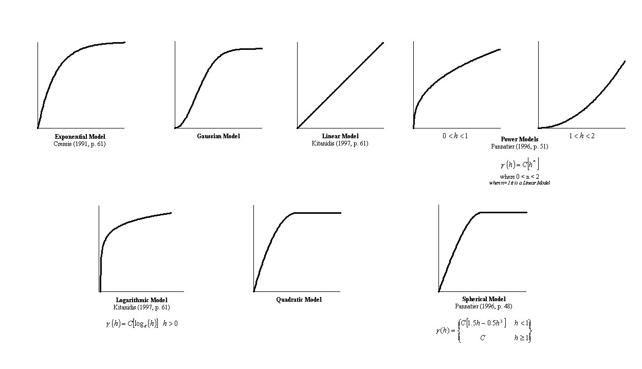
KG_NST_TYPEn defines the variogram to use:

valid values can be:

1-Spherical model of range as KG_NST_APARn

2-exponential model of parameter KG_NST_APARn

3-gaussian model of parameter KG_NST_APARn

4-power model of power KG_NST_APARn

KG_NST_MULTn defines the scale factor for each variogram

KG_NST_AZIMn defines the zimuth angle for the principal direction of continuity (measured clockwise in degrees from Y)

KG_NST_APARn  variogram parameter (see KG_NST_TYPEn)

KG_NST_ANISOn Anisotropy (radius in minor direction at 90 degrees from KG_NST_AZIMn divided by the principal radius in direction KG_NST_AZIMn)

Use KG_DEFAULT passing a value 1 to 4 to setup a default variogram of type 1 to 4 (see KG_NST_TYPEn)

 

References

- François Labelle. Anisotropic Triangular Mesh Generation

Based on Refinement.

- Jim Ruppert. A Delaunay Refinement Algorithm for Quality 2-Dimensional Mesh Generation. Journal or Algorithms 18(3):548-585, May 1995

- A.G.Journel 1978, B.E. Buxton  Apr. 1983, F. Languasco 2002 Ordinary/Simple Kriging of a 2-D Rectangular Grid (FORTRAN 77)

 

 

 

©    Geostru Software