SPECIFICATII TEHNICE DE ELABORARE / PRELUCRARE
Triangulatii limitate / blocate
Principiile unui DTM
Un model digital al terenului este prin definitie un set de date care permite interpolarea unui punct arbitrar al terenului cu o precizie prestabilitã. În acest sens DTM-ul se distinge sibstantial de liniile de contur sau curbe de nivel ale unei hãrti. Curbele de nivel si contururile furnizeazã doar o informatie de altitudine pentru elementul linie; de asemenea, imaginea liniilor de nivel ar trebui sã ofere o idee asupra morfologiei terenului (teren drept, putin ondulat, linii netede ondulate, teren accidentat, linii foarte ondulate, etc.). Liniile curbe de nivel ar trebui sã reprezinte niveluri si mici caracteristici geomorfologice prin intermediul formei lor tipice si a "efectului familie". Acest lucru necesitã, uneori, o exagerare a anumitor forme de relief. Prin urmare, liniile de nivel sunt folosite în special pentru vizualizarea terenului, în timp ce datele pentru un DTM sunt destinate pentru a furniza informatio privind altitudinea si evolutia cotelor din interior în orice punct al terenului într-o formã ce poate fi cititã de un computer. Curbele de nivel obtinude dintr-un dataset al unui DTM nu vor arãta în mod specific morfologia terenului analog celor ale profilelor desenate de un topograf.
Date de bazã pentru un DTM si principii de interpolare. Triangulatia Delaunay
Datele necesare pentru un DTM sunt puncte dispersate (mass points) si linii caracteristice precum break lines, linii structurale ale terenului, talweg, delimitare contururi de zone moarte necartografiabile (dead areas) si altele. O tehnicã foarte de întâlnitã constã în efectuarea unei triangulatii între punctele de sprijin mãsurate. Aceasta înseamnã cã se defineste o seriede triunghiuri în care punctele unghiulare ale vârfurilor sunt puncte dispersate. Foarte des este utilizatã triangulatia Delaunay; în acest caz se alege cercul cel mai mic ce contine doar trei puncte învecinate. În interiorul acestui triunghi se interpoleazã utilizând în general tehnici bilaterale biliniare, dar ocazional se utilizeazã si tehnici bi-cubice. Triangulatia nu poate trece peste o linie caracteristicã. Liniile poligonale frânte de liniile carcteristice sunt întotdeauna utilizate ca linii ale triunghiului ce coincid cu laturile triunghiurilor.
Triangulatii limitate / blocate
Punctele dispersate sau un grid sunt destinate sã reprezinte terenul natural, dar vor reproduce caracteristici diverse ale terenului precum margini si discountinuitãti, amplasamente ale barajelor, însã într-un mod destul de incomplet. Se recomandã deci utilizarea de breack lines sau linii de blocare pentru toate caracteristicile terenului care exced precizia de cotã a DTM-ului.
Se vor indica în mod special zonele cu precizie mai micã acoperite de vegetatie sau alte obstacole, precum si zonele ce nu pot fi mãsurate. În DTM-urile cu precizie mai micã de un metru, ar fi ideal sã fie delimitate si zonele care nu ar trebui marcate pe harta inclusã în DTM, deoarece nu apartin terenului (case, lacuri, etc.).
Se numesc Triangulatii limitate/blocate toate triangulatiile care prevãd elemente structurale pentru care triunghiurile care se vor forma vor urma un criteriu impus de limitare/blocare.
Delaunay Triangulation
We define a triangulation of a finite set of points V in the Euclidean plane to be a maximal planar straight line graph having V as the set of vertices and such that no two edges of the graph properly intersect (i.e. only at their endpoints).
Terrain 5 model terrain using either a regular grid structure or a Triangle Irregular Network (TIN). The advantages of using a TIN are: triangles are simple geometric objects which can be easily manipulated and rendered; TINs are not bound by the regularity constraints of a regular grid and so can approximate any surface at any desired tolerance with a minimal number of polygons; multiple TINs of a single area of terrain can be organised into a hierarchy with respect to their resolution so that they can provide generalizations or details as required by different applications. Of prime importance is that the triangulation is a good approximation to the real-world surface. A second requirement of the triangulation algorithm is that it should produce triangles which are as close to being equiangular as possible. This condition is essential for numerical interpolation since it ensures that the maximum distance from any interior point to a vertex of its enclosing triangle is reduced and it also minimises the aliasing which can arise when long, thin triangles are displayed. Thirdly, we need an algorithm which will produce a unique triangulation of a given set of points so that we generate reproducible and consistent surfaces. A Delaunay Triangulation provides all of the these benefits.
TINs main drawback is that no overhanging features can be represented, but this is usually a minimal concern with terrain. For representing overhanging features, a full blown 3D triangulation must be used.
Terrain 5 uses Delaunay triangulation for immediate use, or as a basis for for mesh smoothing, refining or resampling. Other kinds of mesh can be derived too, like grid meshes or bezier surfaces.
Diagrama Voronoi (cunoscutã si ca Dirichlet sau Theissen tesselation) reprezintã regiunile unui plan care sunt apropiate unui anume punct mai mult decât altele. Diagrama Voronoi are importantã majorã în problemele de geometrie computationalã, de calcul, de exemplu poate fi folositã pentru a rezolva problemele nearest neighbour când este dat un numãr de puncte.
Pentru a sterge datele voronoi produse de program deschideti fereastra "Gestiune DTM" si în panoul "Elemente DTM" apãsati butonul "Cos" de lângã "Voronoi"
Delaunay triangulation and Voronoi tesselation of space
Voronoi Diagrams are closely related to Delaunay Triangulations.
Delaunay (1934) proved that when the dual graph of a Voronoi diagram is drawn with straight lines, it produces a planar triangulation of the Voronoi points P (if no four sites are cocircular). This arrangement is called the Delaunay triangulation of the points.
A Delaunay triangulation is desirable for approximation applications because of its general property that most of its triangles are nearly equiangular and also because it generates a unique triangulation for a given set of points.
The properties of a Voronoi Diagram V(P), of a set of points P={P1,P2,...,Pn}, and its relationship to its corresponding Delaunay Triangulation, are as follows (after O'Rourke 1994):
•each Voronoi region V is convex
•if v is a Voronoi vertex at the junction of regions R(P1), R(P2) and R(P3) then v is the centre of the circle C(v) determined by P1 , P2 and P3
•C(v) is the circumcircle for the Delaunay triangle corresponding to v
•the interior of a circumcircle C(v) contains no points
•if Pj is a nearest neighbour to Pi , then P(i,j) is an edge of V(P)
•there is some circle through Pi and Pj which contains no other points, then (Pi,Pj) is an edge of V(P)
Grids
A grid G is a regurlaly spaced distribution of points Pg() in the Euclidian plane, each point being affected with a height data. A simple mesh can be derived from it as a maximal 3D straight line graph having with Pg() as vertices. Each point Pg() isn't coincident with any original point of P(), but is resulting of a local interpolation of P().
The process of estimating values at evenly spaced grid nodes based on the original irregularly spaced data is called " interpolation". There is no perfect solution to estimate values at each grid node and many techniques are in use. The validity of each depends on the type of data being interpolated and its distribution pattern. Triangulation is most commonly applied to elevation data since it is a technique that uses the slope between data points to estimate new grid values.
Grids are simple structures that can be easyly manipulated, they are, in essence, much like rasters. Unlike TINs, grids are bound by the regularity constraints and so can't approximate any surface at any desired tolerance.
Grid main drawback is it's inhability to represent overhanging features, or any feature topologically shorter than the cell size of the grid. Minimizing the cell size improves terrain representation, but induce an important growth in cells count, hence maximizing rendering time and storage space.
Anisotropic meshing
As in Ruppert's algorithm, the program eliminates "encroached" segments by inserting vertices at their midpoint. The only difference is that encroachment is verified after applying the transformation T assigned to the midpoint of the segment.
Then, the program locks every segment, determines what is the interior region, and starts attacking internal triangles of low quality by refinement (i.e. by inserting new vertices).
When grading is used, the quality of a triangle is defined to be its minimum distorted angle. When grading is not used, large triangles are penalized by dividing the minimum angle by the (distorted) perimeter of the triangle, squared. The power at which the perimeter is raised controls how much importance is given to the size of the triangle versus its shape. The current value was arbitrarily chosen to give pleasing results.
In Ruppert's algorithm, low quality triangles are removed by inserting a vertex at the circumcenter of the triangle. In the isotropic case, the triangle is Delaunay, therefore its circumcircle is empty and the circumcenter is a good place to insert a vertex. Furthermore, a Lemma guarantees that the circumcenter falls in the inside region (using the fact that the input is segment-bounded and that no segment is encroached). However in the anisotropic case there are some problems: the circumcircle is not necessarily empty. The circumcenter may fall arbitrarily close to another vertex or edge, or may even fall in the outside region. The program solves these problems by checking if the nearest neighbor of the circumcenter is a vertex of the triangle in question (as it would be in the isotropic case). If this does not hold, then we walk toward the centroid of the triangle and try again. After some number of consecutive failures, the program finally uses the centroid.
Este vorba despre o tehnicã complexã, stocasticã, de tip exact, si se bazeazã pe teoria variabilelor regionalizate ale lui Krige. Solicitã analiza preliminarã a fenomenului pentru a verifica dacã ipotezele statistice pe care se bazeazã sunt respectate. Este foarte interesantã deoarece furnizeazã o mãsurã a erorii care se comite în interpolare. Tehnica este complexã, si este recomandabilã o aprofundare a argumentelor de statisticã spatialã înainte de a o aplica.
Kriging is a regression based interpolation method that is used to predict unknown values from irregularly spaced known values. It was originally
developed for mapping in the fields of Geology and Geophysics, mining, and photogrammetry.
Kriging takes into account the interdependency of samples that are close to each other while allowing for a certain independence of the sample points.
It avoids the building of a surface based on trends with introduced randomness. Kriging is based on the structural characteristics and behaviour
of spatially located data. Samples taken closer together are expected to be more alike than samples taken farther apart because points that are close together tend to be strongly correlated whereas, points that are far apart tend not to be correlated.
The weights applied to the known values are obtained from a system of linear equations in which the coefficients are the values of variograms or covariance functions. The functions calculate the correlation between known points or known and unknown points. To obtain the function, the variance error must be minimized. The variogram yields the size of the zone of influence, the isotropic nature of the variable, and the continuity of the variable through space.
Custom Variograms
Variograms are the way to drive to the algorithm on its
behaviour. Terrain5 supplies a property KriginParm(key)=value in order to
set/get the required parameter of the variogram. Below the keyword list and their meaning
Enum cKrigingConstants
Key |
Description |
Default value |
KG_DEFAULT |
set default parameters. use this method to test a default variogram (1 to 4) |
|
KG_TRIMMINGMIN |
Minimal trimming limits. |
-1E+21 |
KG_TRIMMINGMAX |
Maximal trimming limit. |
1E+21 |
KG_MINDATAREQ |
Minimum number of data required for kriging |
4 |
KG_MAXSAMPLES |
Maximum number of samples to use in kriging (1 to 120) |
8 |
KG_RADIUS |
Maximum search radius closest max samples will be retained |
Sqr((xmax - xmin)) ^ 2 _ + (ymax - ymin)) ^ 2) (extents of the current mesh/points) |
KG_SIMPLEKRIG |
Indicator for simple kriging (0=No, 1=Yes) |
1 |
KG_SIMPLEKMEAN |
Mean for simple kriging (used if ktype=1) |
2.032 |
KG_ISOTROPICCONST |
Nugget constant (isotropic) |
2 |
KG_NESTEDSTRUCURES |
Number of nested structures (max. 4) |
1 |
KG_NST_TYPE1 |
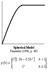
Type of each nested structure: 1. spherical model of range a |
1 |
KG_NST_TYPE2 |
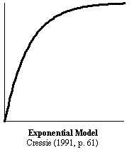
2. exponential model of parameter a. i.e. practical range is 3a |
0 |
KG_NST_TYPE3 |
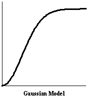
3. gaussian model of parameter a. i.e. practical range is a*sqrt(3) |
0 |
KG_NST_TYPE4 |
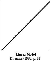
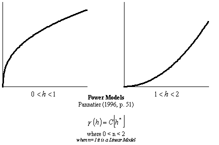
4. power model of power a (a must be > 0 and < 2). if linearmodel,a=1,c=slope |
0 |
KG_NST_MULT1 |
Multiplicative factor of each nested structure |
8 |
KG_NST_MULT2 |
" " |
0 |
KG_NST_MULT3 |
" " |
0 |
KG_NST_MULT4 |
" " |
0 |
KG_NST_AZIM1 |
Azimuth angles for the principal direction of continuity (measured clockwise in degrees from Y) |
0 |
KG_NST_AZIM2 |
" " |
0 |
KG_NST_AZIM3 |
" " |
0 |
KG_NST_AZIM4 |
" " |
0 |
KG_NST_APAR1 |
Parameter "a" of each nested structure. (if KG_NST_TYPEn = 4 must be 0 < KG_NST_APARn < 2) |
1 |
KG_NST_APAR2 |
" " |
0 |
KG_NST_APAR3 |
" " |
0 |
KG_NST_APAR4 |
" " |
0 |
KG_NST_ANISO1 |
KG_NST_ANISOn/KG_NST_APARn = Anisotropy (radius in minor direction at 90 degrees from KG_NST_AZIMn divided by the principal radius in direction KG_NST_AZIMn |
1 |
KG_NST_ANISO2 |
" " |
0 |
KG_NST_ANISO3 |
" " |
0 |
KG_NST_ANISO4 |
" " |
0 |
Variogram Specifications
Trimming limits (KG_TRIMMINGMIN/KG_TRIMMINGMAX) state the range zmin/zmax where the points will be estimated. Points outside that range will be excluded.
kriging system need to know the aumount of cells in which will subvivide the extents of the original data points included into the trimming limits
To do that just set the xCells and yCells on the GetKriging method. Each corner of the cell will be honored by kriging estimation adding a Z height value according with the choosen variogram.
follow all kriging parameters explanation:
Note: we will refer to the original point of the survey as Sample
KG_MINDATAREQ is used to inform Kriging system that will have to process at least n point before to estimate the closest to the current point (or cell corner). Kriging keeps always as samples the original points closest to the current point to esitimate. More points will be used as samples, slower wll be the performances
kriging skips all points far from any found sample, looping throug all remaining samples. KG_MAXSAMPLES will inform the algorithm to exit when a given number of samples has been processed.
KG_RADIUS defines the spherical area where samples will be honored.
use KG_SIMPLEKRIG to use the universal kriging algorithm (0) or simple kriging system (1). By value = 1 evaluate KG_SIMPLEKMEAN which will set the constant Z height all the regions far from sample points.
KG_ISOTROPICCONST means the isotrophism factor while is calculating the covariance between two points
KG_NESTEDSTRUCURES:
A single structure describe the variogram function itself. Terrain supports maximum 4 nested variograms.
KG_NESTEDSTRUCURES describes how many variograms will be used to estimate the covariance between points.
KG_NST_TYPEn,KG_NST_MULTn,KG_NST_AZIMn,KG_NST_APARn,KG_NST_ANISOn are linked to the declared nested structures where n is the index between 1 to KG_NESTEDSTRUCURES
As example if we specify 2 nested structures we will have to setup two variograms using the keywords:
tr.KrigingParm(KG_NESTEDSTRUCTURES)=2
tr.KrigingParm(KG_NST_TYPE1)=1 ' variogram type 1: spherical model
tr.KrigingParm(KG_NST_TYPE2)=3 ' variogram type 3: Gaussian model
ect..
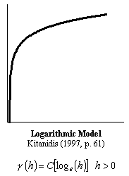
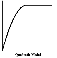
KG_NST_TYPEn defines the variogram to use:
valid values can be:
1-Spherical model of range as KG_NST_APARn
2-exponential model of parameter KG_NST_APARn
3-gaussian model of parameter KG_NST_APARn
4-power model of power KG_NST_APARn
KG_NST_MULTn defines the scale factor for each variogram
KG_NST_AZIMn defines the zimuth angle for the principal direction of continuity (measured clockwise in degrees from Y)
KG_NST_APARn variogram parameter (see KG_NST_TYPEn)
KG_NST_ANISOn Anisotropy (radius in minor direction at 90 degrees from KG_NST_AZIMn divided by the principal radius in direction KG_NST_AZIMn)
Use KG_DEFAULT passing a value 1 to 4 to setup a default variogram of type 1 to 4 (see KG_NST_TYPEn)
- François Labelle. Anisotropic Triangular Mesh Generation
Based on Refinement.
- Jim Ruppert. A Delaunay Refinement Algorithm for Quality 2-Dimensional Mesh Generation. Journal or Algorithms 18(3):548-585, May 1995
- A.G.Journel 1978, B.E. Buxton Apr. 1983, F. Languasco 2002 Ordinary/Simple Kriging of a 2-D Rectangular Grid (FORTRAN 77)
© 2020 Geostru Software